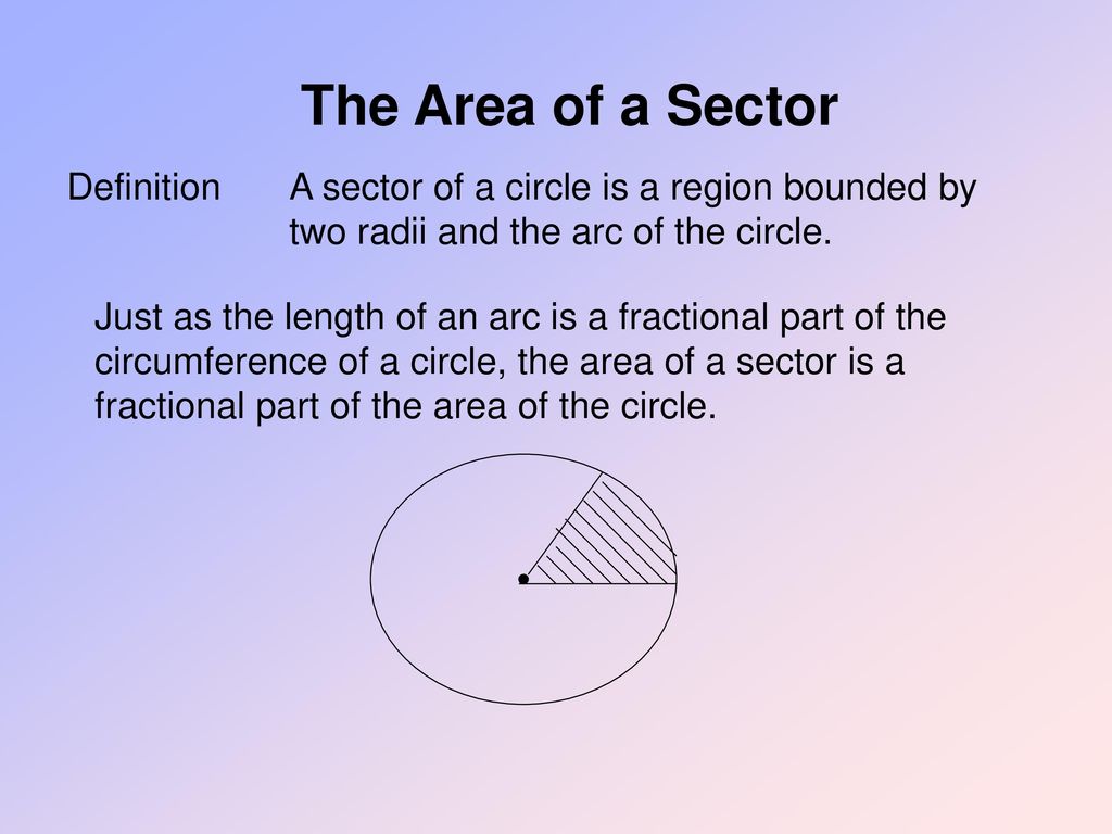
Partitioning in maths definition: FREE Partitioning Explained For Primary School Parents And Kids Worksheets
Posted onWhat is Partitioning in Math? Meaning, Definition, Examples
Here’s an interesting thing about math—you will need it in real-life scenarios, but you may not always have a pencil/pen and paper to solve the calculations.
But by learning partitions in math, you can visualize mathematical problems and solve them in your head—without needing a pencil, paper, or a calculator!
You must be wondering what is Partition in Maths? Let’s see what it is and how we use it.
What Is Partitioning in Math?
Using partitioning in mathematics makes math problems easier as it helps you break down large numbers into smaller units. We can also partition complex shapes to form simple shapes that help make calculations easier.
Partitioning Numbers
a) Addition by Partitioning
Let us think of a number like 956. Now let us add another number, 378, to it. Does this problem seem difficult to solve?
Don’t worry. You will learn a new trick to break down such numbers for easy addition.
Let us start with 956. You can partition this number as
900 + 50 + 6
Here, we have separated the numbers into units, tens, and hundreds.
Similarly, let us partition 378 into units, tens, and hundreds.
300 + 70 + 8
When you write numbers like these, you can visualize them easily in your mind and find it easier to work with them.
Now, you can break down the problem to add 956 and 378:
956 + 378
900 + 50 + 6 + 300 + 70 + 8
Upon adding the tens, units, and hundreds, we get
1200 + 120 + 8
1200 + 128
= 1328
Wasn’t that easy and fun? Let’s learn how to solve more mathematical calculations using partitions.
b) Partitioning in Subtraction
You can also use partitioning for subtracting two numbers.
Let us understand this with an example:
Suppose you have to subtract 42 from 95, you can start by breaking the numbers into units and tens.
So, 95 = 90 + 5
and 42 = 40 + 2
95 − 42 = 90 + 5 − (40 + 2)
= 90 + 5 − 40 − 2
= 90 − 40 + 5 − 2
= 50 + 3
= 53
c) Different Ways of Partitioning Numbers
There are different ways to partition a number.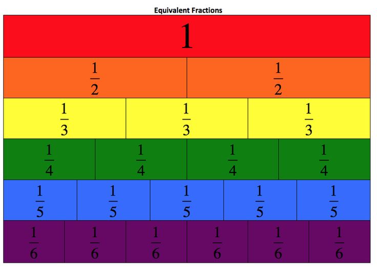 One way is to divide it into hundreds, tens, and units, as we have done above.
However, that’s not the only way.
Depending upon the numbers you are working with, you can divide numbers differently.
Let’s understand this with an example:
Take the number 104. Suppose you have to subtract 4 from it.
In this equation, we should first separate the number into hundreds and units.
So, 104 = 100 + 4
On subtracting 4 from this number, we get
100 + 4 − 4
= 100
However, if you have to subtract 50 from 104, you can break it down as
104 = 50 + 50 + 4
On subtracting 50 from this number, we get
50 + 50 + 4 − 50
= 54
Partitioning of Shapes
Partitioning also refers to dividing shapes or sets into equal or unequal parts.
Let’s talk about shapes first.
A diameter or a line that passes through the center of a circle divides it into two equal parts. Look at the illustration given below:
As you can see here, the circle is divided into two equal parts by line AB. You can represent each part as 1/2 or
The area of each half = 1/2 x area of the circle.
Now, let’s consider a rectangle and partition it into three equal parts.
As seen here, you can represent each part as 1/3 or
The area of each equal part = 1/3 x area of the rectangle
Similarly, if you partition a square into four equal parts, you get an illustration like this:
Here the area of each part = 1/4 x the area of the square.
You can also divide a shape into unequal parts. You can consider the below examples to understand this. Here, each part is not partitioned equally.
Solved Examples
Example 1. Add the numbers 566 and 768 using the partitioning method.
Solution: Let’s first partition 566
566 = 500 + 60 + 6
Similarly,
768 = 700 + 60 + 8
So, 566 + 768
= 500 + 60 + 6 + 700 + 60 + 8
= 500 + 700 + 60 + 60 + 8 + 6
= 1200 + 120 + 14
= 1200 + 134
= 1334
Example 2. Subtract 85 from 420 using the partition method.
Solution: Let’s first partition the numbers into hundreds, tens, and units.
420 − 85
= 400 + 20 − ( 80 + 5)
= 400 + 20 − 80 − 5
= 400 − 60 − 5
= 400 − 65
= 335
Example 3. Calculate the area of each part of a circle divided into two parts by a diameter. The area of the circle is 20 sq. cm.
Solution: We know that a diameter divides a circle into two equal parts.
Thus, the area of each half = 1/2 x the area of the circle
Area of circle = 20 sq. cm.
Area of each half = 1/2 x 20
= 10 sq. cm
Practice Problems
451
381
361
401
Correct answer is: 381
Let us partition 59.
We get 59 = 50 + 9
Let us partition 322.
We get 300 + 20 + 2
On adding both the numbers, we get
50 + 9 + 300 + 20 + 2
= 300 + 50 + 20 + 9 + 2
= 300 + 70 + 11
= 381
811
711
822
801
Correct answer is: 811
876 — 65
= 800 + 70 + 6 − ( 60 + 5)
= 800 + 70 − 60 + 6 − 5
= 800 + 10 + 1
= 811
200
25
50
75
Correct answer is: 50
We know that a diameter divides a circle into two equal parts.
Thus, the area of each half = 1/2 x the area of the circle
Area of the circle = 100 sq. cm.
The area of each half = 1/2 x 100
= 50 sq. cm
15
27.5
50
25
Correct answer is: 25
We know the area of each third = 1/3 x the area of the square
Area of the circle = 75 sq. cm.
The area of each third = 1/3 x 75
= 25 sq. m
Frequently Asked Questions
Is there a formula to calculate the area of unequal parts of a shape?
No, there is no standard formula to calculate the area of unequal parts of a shape.
Can we divide numbers into equal parts?
Yes, you can use fractions to divide numbers into equal parts. You can divide a number by 2 to calculate two equal parts, divide it by 3 to calculate three equal parts, and so on.
Is partitioning necessary for solving all kinds of problems?
No, it is not necessary. However, it does help you simplify numbers and perform easy calculations.
2.3: Partitions of Sets and the Law of Addition
-
- Last updated
- Save as PDF
- Page ID
- 80502
- Al Doerr & Ken Levasseur
- University of Massachusetts Lowell
Partitions
One way of counting the number of students in your class would be to count the number in each row and to add these totals. Of course this problem is simple because there are no duplications, no person is sitting in two different rows. The basic counting technique that you used involves an extremely important first step, namely that of partitioning a set. The concept of a partition must be clearly understood before we proceed further.
Definition \(\PageIndex{1}\): Partition
A partition of set \(A\) is a set of one or more nonempty subsets of \(A\text{:}\) \(A_1, A_2, A_3, \cdots\text{,}\) such that every element of \(A\) is in exactly one set. Symbolically,
- \(\displaystyle A_1 \cup A_2 \cup A_3 \cup \cdots = A\)
- If \(i \neq j\) then \(A_i \cap A_j = \emptyset\)
The subsets in a partition are often referred to as blocks. Note how our definition allows us to partition infinite sets, and to partition a set into an infinite number of subsets. Of course, if \(A\) is finite the number of subsets can be no larger than \(\lvert A \rvert \text{.}\)
Example \(\PageIndex{1}\): Some Partitions of a Four Element Set
Let \(A = \{a, b, c, d\}\text{.}\) Examples of partitions of \(A\) are:
- \(\displaystyle \{\{a\}, \{b\}, \{c, d\}\}\)
- \(\displaystyle \{\{a, b\}, \{c, d\}\}\)
- \(\displaystyle \{\{a\}, \{b\}, \{c\}, \{d\}\}\)
How many others are there, do you suppose?
There are 15 different partitions. The most efficient way to count them all is to classify them by the size of blocks. For example, the partition \(\{\{a\}, \{b\}, \{c, d\}\}\) has block sizes 1, 1, and 2.
Example \(\PageIndex{2}\): Some Integer Partitions
Two examples of partitions of set of integers \(\mathbb{Z}\) are
- \(\{\{n\} \mid n \in \mathbb{Z}\}\) and
- \(\{\{ n \in \mathbb{Z} \mid n < 0\}, \{0\},\{ n \in \mathbb{Z} \mid 0 < n \}\}\text{.}\)
The set of subsets \(\{\{n \in \mathbb{Z} \mid n \geq 0\},\{n \in \mathbb{Z} \mid n \leq 0\}\}\) is not a partition because the two subsets have a nonempty intersection. A second example of a non-partition is \(\{\{n \in \mathbb{Z} \mid \lvert n \rvert = k\} \mid k = -1, 0, 1, 2, \cdots\}\) because one of the blocks, when \(k=-1\) is empty.
One could also think of the concept of partitioning a set as a “packaging problem.” How can one “package” a carton of, say, twenty-four cans? We could use: four six-packs, three eight-packs, two twelve-packs, etc. In all cases: (a) the sum of all cans in all packs must be twenty-four, and (b) a can must be in one and only one pack.
Addition Laws
Theorem \(\PageIndex{1}\): The Basic Law of Addition
If \(A\) is a finite set, and if \(\{A_1,A_2,\ldots ,A_n\}\) is a partition of \(A\) , then
\[\lvert A \rvert = \lvert A_1 \rvert + \lvert A_2 \rvert + \cdots + \lvert A_n \rvert = \sum_{k=1}^n \lvert A_k \rvert \nonumber\]
The basic law of addition can be rephrased as follows: If \(A\) is a finite set where \(A_1 \cup A_2 \cup \cdots \cup A_n = A\) and where \(A_i \cap A_j = \emptyset\) whenever \(i \neq j\text{,}\) then
\begin{equation*} \lvert A \rvert = \lvert A_1 \cup A_2 \cup \cdots \cup A_n \rvert = \lvert A_1 \rvert + \lvert A_2 \rvert + \cdots + \lvert A_n \rvert \end{equation*}
Example \(\PageIndex{3}\): Counting All Students
The number of students in a class could be determined by adding the numbers of students who are freshmen, sophomores, juniors, and seniors, and those who belong to none of these categories. However, you probably couldn’t add the students by major, since some students may have double majors.
Example \(\PageIndex{4}\): Counting Students in Disjoint Classes
The sophomore computer science majors were told they must take one and only one of the following courses that are open only to them: Cryptography, Data Structures, or Javascript. The numbers in each course, respectively, for sophomore CS majors, were 75, 60, 55. How many sophomore CS majors are there? The Law of Addition applies here. There are exactly \(75 + 60 + 55 = 190\) CS majors since the rosters of the three courses listed above would be a partition of the CS majors.
Example \(\PageIndex{5}\): Counting Students in Non-Disjoint Classes
It was determined that all junior computer science majors take at least one of the following courses: Algorithms, Logic Design, and Compiler Construction. Assume the number in each course was 75, 60 and 55, respectively for the three courses listed. Further investigation indicated ten juniors took all three courses, twenty-five took Algorithms and Logic Design, twelve took Algorithms and Compiler Construction, and fifteen took Logic Design and Compiler Construction. How many junior C.S. majors are there?
Example \(\PageIndex{4}\) was a simple application of the law of addition, however in this example some students are taking two or more courses, so a simple application of the law of addition would lead to double or triple counting. We rephrase information in the language of sets to describe the situation more explicitly.
\(A\) = the set of all junior computer science majors
\(A_1\) = the set of all junior computer science majors who took Algorithms
\(A_2\) = the set of all junior computer science majors who took Logic Design
\(A_3\) = the set of all junior computer science majors who took Compiler Construction
Since all junior CS majors must take at least one of the courses, the number we want is:
\begin{equation*} \lvert A \rvert = \lvert A_1 \cup A_2 \cup A_3 \rvert = \lvert A_1 \rvert + \lvert A_2 \rvert + \lvert A_3 \rvert — \textrm{repeats}. \end{equation*}
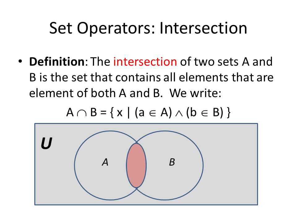
A Venn diagram is helpful to visualize the problem. In this case the universal set \(U\) can stand for all students in the university.
Figure \(\PageIndex{1}\): Venn Diagram
We see that the whole universal set is naturally partitioned into subsets that are labeled by the numbers 1 through 8, and the set \(A\) is partitioned into subsets labeled 1 through 7. The region labeled 8 represents all students who are not junior CS majors. Note also that students in the subsets labeled 2, 3, and 4 are double counted, and those in the subset labeled 1 are triple counted. To adjust, we must subtract the numbers in regions 2, 3 and 4. This can be done by subtracting the numbers in the intersections of each pair of sets. However, the individuals in region 1 will have been removed three times, just as they had been originally added three times. Therefore, we must finally add their number back in.
\begin{equation*} \begin{split} \lvert A \rvert & = \lvert A_1 \cup A_2 \cup A_3 \rvert \\ & = \lvert A_1 \rvert + \lvert A_2 \rvert + \lvert A_3 \rvert — \textrm{repeats} \\ & = \lvert A_1 \rvert + \lvert A_2 \rvert + \lvert A_3 \rvert — \textrm{duplicates} + \textrm{triplicates} \\ & = \lvert A_1 \rvert + \lvert A_2 \rvert + \lvert A_3 \rvert — \left(\lvert A_1 \cap A_2 \rvert + \lvert A_1 \cap A_3 \rvert+ \lvert A_2 \cap A_3 \rvert \right) + \lvert A_1 \cap A_2 \cap A_3 \rvert \\ & = 75 + 60 + 55 — 25 — 12 — 15 + 10 = 148 \end{split} \end{equation*}
The ideas used in this latest example gives rise to a basic counting technique:
Theorem \(\PageIndex{2}\): Laws of Inclusion-Exclusion
Given finite sets \(A_1, A_2, A_3\text{,}\) then
- The Two Set Inclusion-Exclusion Law:
\begin{equation*} \lvert A_1 \cup A_2 \rvert =\lvert A_1 \rvert + \lvert A_2 \rvert — \lvert A_1 \cap A_2 \rvert \end{equation*} - The Three Set Inclusion-Exclusion Law:
\begin{equation*} \begin{split} \lvert A_1 \cup A_2 \cup A_3 \rvert & =\lvert A_1 \rvert + \lvert A_2 \rvert + \lvert A_3 \rvert\\ &\quad — (\lvert A_1 \cap A_2 \rvert + \lvert A_1 \cap A_3 \rvert+ \lvert A_2 \cap A_3 \rvert)\\ &\quad + \lvert A_1 \cap A_2 \cap A_3 \rvert \end{split} \end{equation*}
The inclusion-exclusion laws extend to more than three sets, as will be explored in the exercises. c\) . Use the resulting diagram and the definition of partition to convince yourself that the subset of these four subsets that are nonempty form a partition of \(U\text{.}\)
Exercise \(\PageIndex{5}\)
Show that \(\{\{2 n \mid n \in \mathbb{Z}\}, \{2 n + 1 \mid n \in \mathbb{Z}\}\}\) is a partition of \(\mathbb{Z}\text{.}\) Describe this partition using only words.
- Answer
-
The first subset is all the even integers and the second is all the odd integers. These two sets do not intersect and they cover the integers completely.
Exercise \(\PageIndex{6}\)
- A group of 30 students were surveyed and it was found that 18 of them took Calculus and 12 took Physics. If all students took at least one course, how many took both Calculus and Physics? Illustrate using a Venn diagram.
- What is the answer to the question in part (a) if five students did not take either of the two courses? Illustrate using a Venn diagram.

Exercise \(\PageIndex{7}\)
A survey of 90 people, 47 of them played tennis and 42 of them swam. If 17 of them participated in both activities, how many of them participated in neither?
- Answer
-
Since 17 participated in both activities, 30 of the tennis players only played tennis and 25 of the swimmers only swam. Therefore, \(17+30+25=72\) of those who were surveyed participated in an activity and so 18 did not.
Exercise \(\PageIndex{8}\)
A survey of 300 people found that 60 owned an iPhone, 75 owned a Blackberry, and 30 owned an Android phone. Furthermore, 40 owned both an iPhone and a Blackberry, 12 owned both an iPhone and an Android phone, and 8 owned a Blackberry and an Android phone. Finally, 3 owned all three phones.
- How many people surveyed owned none of the three phones?
- How many people owned a Blackberry but not an iPhone?
- How many owned a Blackberry but not an Android?
Exercise \(\PageIndex{9}\)
Regarding Theorem \(\PageIndex{2}\),
- Use the two set inclusion-exclusion law to derive the three set inclusion-exclusion law. Note: A knowledge of basic set laws is needed for this exercise.
- State and derive the inclusion-exclusion law for four sets.
 Note: A knowledge of basic set laws is needed for this exercise.
- Answer
-
We assume that \(\lvert A_1 \cup A_2 \rvert = \lvert A_1 \rvert +\lvert A_2\rvert -\lvert A_1\cap A_2\rvert \text{.}\)
\begin{equation*} \begin{split} \lvert A_1 \cup A_2\cup A_3 \rvert & =\lvert (A_1\cup A_2) \cup A_3 \rvert \quad Why?\\ & = \lvert A_1\cup A_2\rvert +\lvert A_3 \rvert -\lvert (A_1\cup A_2)\cap A_3\rvert \quad Why? \\ & =\lvert (A_1\cup A_2\rvert +\lvert A_3\rvert -\lvert (A_1\cap A_3)\cup (A_2\cap A_3)\rvert \quad Why?\\ & =\lvert A_1\rvert +\lvert A_2\rvert -\lvert A_1\cap A_2\rvert +\lvert A_3\rvert \\ & \quad -(\lvert A_1\cap A_3\rvert +\lvert A_2\cap A_3\rvert -\lvert (A_1\cap A_3)\cap (A_2\cap A_3)\rvert\quad Why?\\ & =\lvert A_1\rvert +\lvert A_2\rvert +\lvert A_3\rvert -\lvert A_1\cap A_2\rvert -\lvert A_1\cap A_3\rvert\\ & \quad -\lvert A_2\cap A_3\rvert +\lvert A_1\cap A_2\cap A_3\rvert \quad Why? \end{split} \end{equation*}
The law for four sets is
\begin{equation*} \begin{split} \lvert A_1\cup A_2\cup A_3\cup A_4\rvert & =\lvert A_1\rvert +\lvert A_2\rvert +\lvert A_3\rvert +\lvert A_4\rvert\\ & \quad -\lvert A_1\cap A_2\rvert -\lvert A_1\cap A_3\rvert -\lvert A_1\cap A_4\rvert \\ & \quad \quad -\lvert A_2\cap A_3\rvert -\lvert A_2\cap A_4\rvert -\lvert A_3\cap A_4\rvert \\ & \quad +\lvert A_1\cap A_2\cap A_3\rvert +\lvert A_1\cap A_2\cap A_4\rvert \\ & \quad \quad +\lvert A_1\cap A_3\cap A_4\rvert +\lvert A_2\cap A_3\cap A_4\rvert \\ & \quad -\lvert A_1\cap A_2\cap A_3\cap A_4\rvert \end{split} \end{equation*}
Derivation:
\begin{equation*} \begin{split} \lvert A_1\cup A_2\cup A_3\cup A_4\rvert & = \lvert (A_1\cup A_2\cup A_3)\cup A_4\rvert \\ & = \lvert (A_1\cup A_2\cup A_3\rvert +\lvert A_4\rvert -\lvert (A_1\cup A_2\cup A_3)\cap A_4\rvert\\ & = \lvert (A_1\cup A_2\cup A_3\rvert +\lvert A_4\rvert \\ & \quad -\lvert (A_1\cap A_4)\cup (A_2\cap A_4)\cup (A_3\cap A_4)\rvert \\ & = \lvert A_1\rvert +\lvert A_2\rvert +\lvert A_3\rvert -\lvert A_1\cap A_2\rvert -\lvert A_1\cap A_3\rvert \\ & \quad -\lvert A_2\cap A_3\rvert +\lvert A_1\cap A_2\cap A_3\rvert +\lvert A_4\rvert -\lvert A_1\cap A_4\rvert \\ & \quad+\lvert A_2\cap A_4\rvert +\lvert A_3\cap A_4\rvert -\lvert (A_1\cap A_4)\cap (A_2\cap A_4)\rvert \\ & \quad -\lvert (A_1\cap A_4)\cap (A_3\cap A_4)\rvert -\lvert (A_2\cap A_4)\cap (A_3\cap A_4)\rvert \\ & \quad +\lvert (A_1\cap A_4)\cap (A_2\cap A_4)\cap (A_3\cap A_4)\rvert \\ & =\lvert A_1\rvert +\lvert A_2\rvert +\lvert A_3\rvert +\lvert A_4\rvert -\lvert A_1\cap A_2\rvert -\lvert A_1\cap A_3\rvert \\ & \quad -\lvert A_2\cap A_3\rvert -\lvert A_1\cap A_4\rvert -\lvert A_2\cap A_4\rvert \quad -\lvert A_3\cap A_4\rvert \\ & \quad +\lvert A_1\cap A_2\cap A_3\rvert +\lvert A_1\cap A_2\cap A_4\rvert \\ & \quad +\lvert A_1\cap A_3\cap A_4\rvert +\lvert A_2\cap A_3\cap A_4\rvert \\ & \quad -\lvert A_1\cap A_2 \cap A_3\cap A_4\rvert \end{split} \end{equation*}
Exercise \(\PageIndex{10}\)
To complete your spring schedule, you must add Calculus and Physics.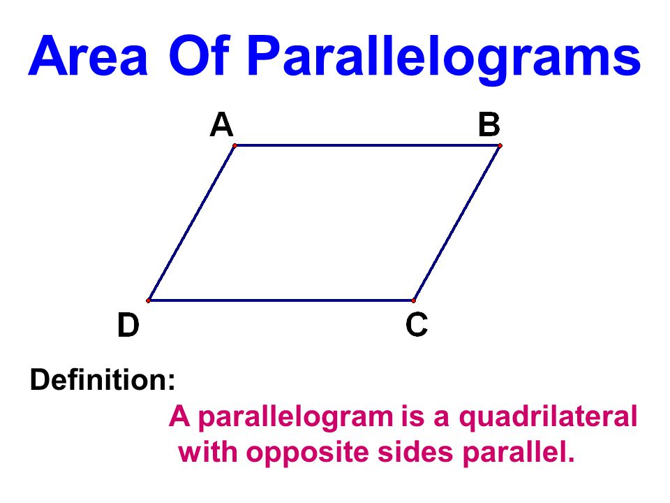 At 9:30, there are three Calculus sections and two Physics sections; while at 11:30, there are two Calculus sections and three Physics sections. How many ways can you complete your schedule if your only open periods are 9:30 and 11:30?
Exercise \(\PageIndex{11}\)
The definition of \(\mathbb{Q} = \{a/b \mid a, b \in \mathbb{Z}, b \neq 0\}\) given in Chapter 1 is awkward. If we use the definition to list elements in \(\mathbb{Q}\text{,}\) we will have duplications such as \(\frac{1}{2}\text{,}\) \(\frac{-2}{-4}\) and \(\frac{300}{600}\) Try to write a more precise definition of the rational numbers so that there is no duplication of elements.
- Answer
-
Partition the set of fractions into blocks, where each block contains fractions that are numerically equivalent. Describe how you would determine whether two fractions belong to the same block. Redefine the rational numbers to be this partition. Each rational number is a set of fractions.

- Back to top
-
- Was this article helpful?
-
- Article type
- Section or Page
- Author
- Al Doerr & Ken Levasseur
- License
- CC BY-NC-SA
- Show Page TOC
- no
-
- Tags
-
Partitions | NZ Maths
Use the resource finder
OR
Username
Password
- Forgot password ?
- Register
Purpose
This unit is about partitioning whole numbers. It focuses on partitioning numbers to “make a ten” or a decade when adding whole numbers, for example 8 + 6 can be solved as (8 + 2) + 4. The unit uses measurement as a context.
Achievement Objectives
NA2-7: Generalise that whole numbers can be partitioned in many ways.
AO elaboration and other teaching resources
Specific Learning Outcomes
- Partition numbers less than 10.
- Know and use «teen» facts.
- Solve addition problems by making a ten, or making a decade.
- Solve addition problems involving measurements.
Description of Mathematics
Students at Level Two should understand that numbers are counts that can be split in ways that make the operations of addition, subtraction, multiplication and division easier. From Level One students will understand that counting a set tells how many objects are in the set. At Level Two they are learning that the count of a set can be partitioned and that the count of each subset tells how many objects are in that subset. Students also need to understand that partitions of a count can be recombined. For example, a count of ten can be partitioned into 1 and 9, 2 and 8, 3 and 7, etc.
It is important that students understand that because there are many ways to partition a number and they will need to choice the best partition to suit the question. In this unit we focus on making partitions that allow numbers to make a ten. For example 8 + 6, the 6 can be partitioned to 2 + 4, the 2 then combines with 8 to make a ten 8 + 2, + 4. For this reason teachers should ensure that they select questions that are best solved using the «make a ten» strategy as opposed to partitioning to make doubles. For example, 8 + 7 also encourages the strategy 7 + 7 + 1 rather than 8 + 2 + 5.
This unit uses the context of measurement. Examples and problems should use like measures, and students should be encouraged to write the units when they give an answer, for example 8m + 5m = 13m.
Required Resource Materials
- Plastic animals
- Unifix cubes
- Tens Frames
- Small bottle/s
- Ice cube tray/s
- Numeral flip strip (Material Master 4-2)
- Packet of 10 items, and single items (e. g pens)
 g pens)
Activity
Session 1
In this session students investigate the fact that whole numbers can be partitioned in a number of ways.
- Show the students a bag of 8 plastic farm animals and a piece of paper with 2 rectangles drawn to represent 2 paddocks. Tell the students you are going to find all the ways of splitting the animals between the 2 paddocks.
- Ask the students:
How many animals should I put in the first paddock? (Put that number (for example, 3) in that paddock and the rest in the second paddock)
How many animals are in the second paddock? Make sure the students understand there is still 8 animals. - Record for the students 3 + 5 = 8.
- Continue working with the students to find all the pairs of number that add to 8. For example, 6 + 2 and 2 + 6.
- Show the students a length of 7 unifix cubes. Work with students to find different ways of partitioning the 7 cubes. Record the partitions, for example 4 + 3.
- Students can continue to explore partitioning numbers for numbers up to 10. Students can work in pairs or individuals to partition the number and record the results. Students can use unifix cubes, sets of counters, strips of squared paper as materials to help. Students who know the basic addition and subtraction facts to 10 will be able to partition numbers without materials.
Session 2
In this session students investigate that partitioning teen numbers using the number ten. It is easiest to start by making teens numbers as 10 + x.
|
Object |
Length |
Splits |
|
Sellotape dispenser |
|
10 cm + cm |
|
Duster |
|
|
|
Stapler |
|
|
|
Notebook |
|
|
|
etc |
|
|
- Show the students a packet of pens (or item that comes in packs of 10) and 5 single pens.
- Ask the students: how many pens do I have? (Students may count on 11, 12, 13 etc,)
- Record the answer as 10 + 5 = 15. Do several more examples.
- Show the students two tens frames, one complete with 10 dots and another with 6 dots. Ask the students how many dots are there? Again record the answer as 10 + 6 = 16. Using the tens frames work with the students to do solve more examples.
- Students also need to be able to understand that teens numbers can be partitioned. Tell the students that in today’s session the numbers are going to be split into 10 and something.
- Show the students two blank tens frame and a pile of 16 counters. Tell the students you know there are more than 10 counters in the pile, but how many more? Put the counters on the tens frames.
- Ask the students: 16 can be split into 10 plus what?
- Record the answer as 16 = 10 + 6.
- Name some objects in the classroom that are between 11 and 20 cm. Ask the students to measure the length using their ruler and record the answer on the table.
- Other measurement contexts can be used to provide practice activities. For example, capacity. Pour enough water into a bottle to make about 18 ice cubes. Ask the students to pour the water into the ice cubes tray and count how many ice cubes it would make. Ask the students to write their answer as 10 + ? Bottles with different amounts of water can be used.
 Ask the students to measure the length using their ruler and record the answer on the table.
Session 3
In this session students solve addition problems by partitioning numbers. They use the strategy “make a ten”.
- Show the students a number strip (see Resources) from 0 – 20 and colour in the 10 square. Place 7 counters on the strip. Tell the students that you are going to use the number strip to help add 7 + 5. Show the students a group of 5 counters.
- Ask the students: how many counters will it take to get to 10? (3)
- Put on the 3 counters then ask the students:
How many counters are there to add on? (2)
What does 10 and 2 make?
What two numbers did we split the 5 into? (3 +2)
Why did we chose 3, then 2? (To make it up to 10) - Write the problem 8 + 6 for the students to see.
Ask the students:
How many counters would be need to get to 10? (2)
How many counters are there still to add on? (4)
What is 10 plus 4? (14)
Check the answer using counters and the number strip. - Draw a number line and pose the question 7 + 4.
Start at the 7, ask the students:
How many jumps do we need to add on? (4)
How many jumps is it to get to 10? (3)
How many left over from the 4? (1)
What is 10 and 1? (11) - Students can practise using the make a ten strategy on number lines. Pose questions using the context of measurement and encourage students to write the correct units beside the answer. Possible questions are:
- The bucket had 9 litres in it and Kitiona poured in another 6 litres. How many litres are now in the bucket?
- Anna put 7 cups of juice on the tray and Kiri added another 5 cups to the tray. How many cups were there altogether?
- The temperature was 8oC and it rose 3 degrees during the morning. What is the temperature now?
- Rangi left George’s house and ran 8 minutes then walked for 5 minutes before he got home. How many minutes did it take him to get home?
- Mum bought 7 kilograms of kumara and 4 kilograms of carrots. How much did the vegetables weigh?
 How many cups were there altogether?
Session 4
In this session students solve addition problems by partitioning numbers. They will solve problems that involve adding a 1 digit number to a 2 digit number. The “make a ten” strategy is applied to decade numbers, for example 28 + 7 is solved by making it up to 30 and then adding the remaining 5.
- Pose the problem: If the plant was 37cm tall and it grew 8cm, how tall is it now? Show the students a number line that ranges from 0 – 100, with the 10s numbers coloured in.
- Ask the students: Using the make a ten strategy we used yesterday, how could we solve this problem?
- Work with students to jump 3 to get to 40, then jump the remaining 5 to get to 45.
- Pose the question: The suitcase weighed 17 kilograms and the backpack weighed 5 kilograms. How much did the luggage weigh altogether?
Show the students how they can draw a number line to suit the question.
Ask the students: what numbers are we adding together? (17 and 5)
Draw a line and the number 17 underneath.
Ask the students: what number can be jump to from here? (20)
how many jumps is that? (3)
how many of the 5 are left? (2)
What is the answer? (22) - Students can practise using the make a decade strategy on their own number lines. Pose questions using the context of measurement and encourage students to write the correct units beside the answer. Possible questions are:
- Jane was going home on the bus. The bus took 26 minutes then she walked for 8 minutes. How long did it take for Jane to get home?
- Peni’s plant was 48cm tall. It grew another 7cm. How tall is Peni’s plant now?
- Dad went to the garden shop and bought 16kg of compost and 7kg of fertilizer. How much did it all weigh?
- The painter had 65 litres of paint and he bought another 8 litres. How much paint does he now have?
- In the first three weeks of October Wellington had 88mm of rainfall, in the rest of the month another 7mm fell. How much rain is that altogether?
 How much did it all weigh?
Session 5
In this session you may wish to continue to give the students opportunities to practise addition partitioning with the make a ten or make a decade strategy. Problems could focus around one measurement theme, for example length. Or problems could focus around a theme such as camping and involve more than one measurement context, for example, weight of packs, time spent on activities, capacity of shower water, length of washing lines, etc.
Alternatively, you may wish to use the formats of session 3 and 4 to show students how this partitioning strategy can be used to solve subtraction problems. For example, 44 – 7, it takes 4 jumps to get back to 40, then the remaining 3 jumps takes us back to 37.
Home Link
Dear Parents and Whānau,
This week in maths your child has been learning to use a number line and to make jumps to 10 to work out addition questions. Ask them to show you how they jump to the 10 first to solve 8 + 5.
You could pose some other similar problems, like 7 + 4, 9 + 6 and have them use jumps to 10 to solve them. Thank you for your help.
Add to plan
Level Two
Counting Partitions
\( \def\negchoose#1#2{\genfrac{[}{]}{0pt}{}{#1}{#2}_{-1}}
\newcommand{\mchoose}[2]{\left(\!\binom{#1}{#2}\!\right)}
\newcommand{\cycle}[1]{\arraycolsep 5 pt
\left(\begin{array}#1\end{array}\right)}
\newcommand{\importantarrow}{\Rightarrow}
\newcommand{\qchoose}[2]{\left[{#1\atop#2}\right]_q}
\newcommand{\bp}{
\begin{enumerate}{\setcounter{enumi}{\value{problemnumber}}}}
\newcommand{\ep}{\setcounter{problemnumber}{\value{enumi}}
\end{enumerate}}
\newcommand{\ignore}[1]{}
\renewcommand{\bottomfraction}{. 8}
8}
\renewcommand{\topfraction}{.8}
\newcommand{\apple}{\text{🍎}}
\newcommand{\ap}{\apple}
\newcommand{\banana}{\text{🍌}}
\newcommand{\ba}{\banana}
\newcommand{\pear}{\text{🍐}}
\newcommand{\pe}{\pear}
\DeclareMathOperator{\Fix}{Fix}
\DeclareMathOperator{\Orb}{Orb}
\newcommand{\F}{\mathcal{F}}
\newcommand{\alert}{\fbox}
\def\d{\displaystyle}
\def\course{Math 228}
\newcommand{\f}[1]{\mathfrak #1}
\newcommand{\s}[1]{\mathscr #1}
\def\N{\mathbb N}
\def\B{\mathbf{B}}
\def\circleA{(-.5,0) circle (1)}
\def\Z{\mathbb Z}
\def\circleAlabel{(-1.5,.6) node[above]{$A$}}
\def\Q{\mathbb Q}
\def\circleB{(.5,0) circle (1)}
\def\R{\mathbb R}
\def\circleBlabel{(1.5,.6) node[above]{$B$}}
\def\C{\mathbb C}
\def\circleC{(0,-1) circle (1)}
\def\F{\mathbb F}
\def\circleClabel{(.5,-2) node[right]{$C$}}
\def\A{\mathbb A}
\def\twosetbox{(-2,-1.5) rectangle (2,1.5)}
\def\X{\mathbb X}
\def\threesetbox{(-2,-2.5) rectangle (2,1.5)}
\def\E{\mathbb E}
\def\O{\mathbb O}
\def\U{\mathcal U}
\def\pow{\mathcal P}
\def\inv{^{-1}}
\def\nrml{\triangleleft}
\def\st{:}
\def\~{\widetilde}
\def\rem{\mathcal R}
\def\sigalg{$\sigma$-algebra }
\def\Gal{\mbox{Gal}}
\def\iff{\leftrightarrow}
\def\Iff{\Leftrightarrow}
\def\land{\wedge}
\def\And{\bigwedge}
\def\entry{\entry}
\def\AAnd{\d\bigwedge\mkern-18mu\bigwedge}
\def\Vee{\bigvee}
\def\VVee{\d\Vee\mkern-18mu\Vee}
\def\imp{\rightarrow}
\def\Imp{\Rightarrow}
\def\Fi{\Leftarrow}
\def\var{\mbox{var}}
\def\Th{\mbox{Th}}
\def\entry{\entry}
\def\sat{\mbox{Sat}}
\def\con{\mbox{Con}}
\def\iffmodels{\bmodels\models}
\def\dbland{\bigwedge \!\!\bigwedge}
\def\dom{\mbox{dom}}
\def\rng{\mbox{range}}
\def\isom{\cong}
\DeclareMathOperator{\wgt}{wgt}
\newcommand{\vtx}[2]{node[fill,circle,inner sep=0pt, minimum size=4pt,label=#1:#2]{}}
\newcommand{\va}[1]{\vtx{above}{#1}}
\newcommand{\vb}[1]{\vtx{below}{#1}}
\newcommand{\vr}[1]{\vtx{right}{#1}}
\newcommand{\vl}[1]{\vtx{left}{#1}}
\renewcommand{\v}{\vtx{above}{}}
\def\circleA{(-.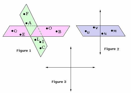 5,0) circle (1)}
\def\circleAlabel{(-1.5,.6) node[above]{$A$}}
\def\circleB{(.5,0) circle (1)}
\def\circleBlabel{(1.5,.6) node[above]{$B$}}
\def\circleC{(0,-1) circle (1)}
\def\circleClabel{(.5,-2) node[right]{$C$}}
\def\twosetbox{(-2,-1.4) rectangle (2,1.4)}
\def\threesetbox{(-2.5,-2.4) rectangle (2.5,1.4)}
\def\ansfilename{practice-answers}
\def\shadowprops{{fill=black!50,shadow xshift=0.5ex,shadow yshift=0.5ex,path fading={circle with fuzzy edge 10 percent}}}
\newcommand{\hexbox}[3]{
\def\x{-cos{30}*\r*#1+cos{30}*#2*\r*2}
\def\y{-\r*#1-sin{30}*\r*#1}
\draw (\x,\y) +(90:\r) — +(30:\r) — +(-30:\r) — +(-90:\r) — +(-150:\r) — +(150:\r) — cycle;
\draw (\x,\y) node{#3};
}
\newcommand{\card}[1]{\left| #1 \right|}
\newcommand{\twoline}[2]{\begin{pmatrix}#1 \\ #2 \end{pmatrix}}
\newcommand{\lt}{<}
\newcommand{\gt}{>}
\newcommand{\amp}{&}
\)
¶
In Section 2.3 we considered some ways to distribute items to recipients. Most basic counting formulas can be thought of as counting the number of ways to distribute either distinct or identical items to distinct recipients. k\) ways, if recipients can receive any number of items, or \(P(n,k)\) ways if recipients can receive at most one item. If the items are identical, the corresponding number of ways to distribute them are \(\mchoose{n}{k}\) and \(\binom{n}{k}\text{.}\)
What if the recipients are not distinct? Say we wish to distribute \(k\) books (either distinct or identical) to \(n\) identical boxes. This is a perfectly natural extension, but we will see the answer is not. First, let’s get a feel for what this might look like for some small values of \(k\) and \(n\text{.}\)
Activity196
Suppose you have \(3\) distinct books you want to put in \(5\) identical boxes.
(a)
How many ways can you do this if each box can have at most one book?
(b)
How many ways can you do this if any box can have any number of books? You might want to consider three cases: one, two, or three boxes are used. Assume we do not care about the order in which the books are placed inside boxes.
(c)
Describe the outcomes we are counting in abstract mathematical terms. What sort of mathematical objects are we counting?
Activity197
Suppose you have \(3\) identical books you want to put in \(5\) identical boxes.
(a)
How many ways can you do this if each box can have at most one book?
(b)
How many ways can you do this if any box can have any number of books? Again, you should consider three cases.
(c)
What mathematical objects are we counting here?
Subsection3.1.1Partitions of Sets
¶
Recall that a partition of a set \(A\) is a set of subsets of \(A\) such that every element of \(A\) is in exactly one of the subsets. Sometimes we will call the subsets that make up a partition blocks.
Definition3.1.1
Denote by \(S(k,n)\) the number of partitions of \([k]\) into exactly \(n\) subsets. We call \(S(k,n)\) a Stirling number (of the second kind).
Note that we write \(S(k,n)\) instead of \(S(n,k)\) here because we try to use \(k\) for the number of elements being distributed and \(n\) for the number of recipients. When other books use \(S(n,k)\text{,}\) they mean the number of partitions of \([n]\) into exactly \(k\) blocks. This is the same definition as we give, but with renamed variables, formulas might look different.
For example, consider how to partition \([3]\) into exactly two sets:
\begin{equation*}
\{1,2\}, \{3\} \qquad \qquad \{1,3\},\{2\} \qquad \qquad \{2,3\},\{1\}
\end{equation*}
and that is all, so \(S(3,2) = 3\text{.}\) We do not care about the order the elements appear in each block, nor the order in which the blocks appear. Thus we see the Stirling numbers count the number of ways to distribute \(k\) distinct items to \(n\) identical recipients so that each recipient gets at least one item.
Activity198
Get to know the Stirling numbers by finding some. List the set of partitions and count them.
(a)
Find \(S(3,1)\text{,}\) \(S(4,1)\) and \(S(k,1)\text{.}\)
(b)
Compute \(S(2,2)\text{,}\) \(S(3,2)\) and \(S(4,2)\text{.}\) Find a formula for \(S(k,2)\) and prove it is correct.
(c)
Compute \(S(3,3)\text{,}\) and \(S(4,3)\text{.}\)
(d)
Find formulas and give proofs for \(S(k,k)\) and \(S(k,k — 1)\text{.}\)
Hint
What are the possible sizes of parts?
We can arrange the Stirling numbers into a triangle (called Stirlings second triangle). The first five rows are shown below. The entries are indexed differently than in Pascal’s triangle: the top 1 represents \(S(1,1)\text{,}\) so for example, \(S(5,2) = 15\text{.}\)
| 1 | ||||||||
| 1 | 1 | |||||||
| 1 | 3 | 1 | ||||||
| 1 | 7 | 6 | 1 | |||||
| 1 | 15 | 25 | 10 | 1 |
How were these found? Sure, I could have written out all 25 of the partitions of \([5]\) into exactly \(3\) blocks, but I didn’t. Could there be some way to get 25 from the entries above it? That is, what is the recurrence relation among the Stirling numbers?
Activity199
(a)
Write down (if you haven’t already) all 6 partitions of \([4]\) into \(3\) blocks. Break these into two cases by where 4 is: is 4 is solitary confinement (in a singleton set) or does he have a cellmate?
(b)
How could you take the \(S(4,2) = 7\) partitions of \([4]\) into 2 sets and the \(S(4,3) = 6\) partitions of \([4]\) into 3 sets and form all the \(S(5,3) = 25\) partitions of \([5]\) into \(3\) sets?
Activity200
Now generalize. In a partition of the set \([k]\text{,}\) the number \(k\) is either in a block by itself, or it is not. Find a two variable recurrence for \(S(n,k)\text{,}\) valid for \(n\) and \(k\) larger than one.
Hint
The number of partitions of \([k]\) into \(n\) parts in which \(k\) is not in a block relates to the number of partitions of \(k-1\) into some number of blocks in a way that involves \(n\text{. }\) With this in mind, review how you proved Pascal’s (recurrence) equation.
Activity201
Find a recurrence for the Lah numbers \(L(k,n)\) similar to the one in Activity 200.
Hint
To see how many broken permutations of a \(k\) element set into \(n\) parts do not have \(k\) is a part by itself, ask yourself how many broken permutations of \([7]\) result from adding 7 to the one of the two permutations in the broken permutation \(\{14, 2356\}\text{.}\)
Activity202
Extend Stirling’s triangle enough to allow you to answer the following question and answer it. (Don’t fill in the rows all the way; the work becomes quite tedious if you do. Only fill in what you need to answer this question.) A caterer is preparing three bag lunches for hikers. The caterer has nine different sandwiches. In how many ways can these nine sandwiches be distributed into three identical lunch bags so that each bag gets at least one?
We have often thought of counting problems as asking about how many functions there are from a \(k\)-elements set to an \(n\)-element set. k\) for all functions and \(P(n,k)\) for injective functions. What about surjective functions? There is a reason we haven’t asked this question yet, but now we can at least get an expression for the number of surjections in terms of Stirling numbers.
Activity203
Given a function \(f\) from a \(k\)-element set \(K\) to an \(n\)-element set, we can define a partition of \(K\) by putting \(x\) and \(y\) in the same block of the partition if and only if \(f(x)=f(y)\text{.}\) How many blocks does the partition have if \(f\) is surjective? How is the number of functions from a \(k\)-element set onto an \(n\)-element set related to a Stirling number? Be as precise in your answer as you can.
Hint
You can think of a function as assigning values to the blocks of its partition. If you permute the values assigned to the blocks, do you always change the function?
We do not have an explicit formula for either the number of surjections or for \(S(k,n)\) yet, but note that if we could find either, we would now have both. We will see one approach to this in Section 3.2.
Activity204
Each function from a \(k\)-element set \(K\) to an \(n\)-element set \(N\) is a function from \(K\) onto some subset of \(N\text{.}\) If \(J\) is a subset of \(N\) of size \(j\text{,}\) you know how to compute the number of functions that map onto \(J\) in terms of Stirling numbers. Suppose you add the number of functions mapping onto \(J\) over all possible subsets \(J\) of \(N\text{.}\) What simple value should this sum equal? Write the equation this gives you.
Hint
When you add the number of functions mapping onto \(J\) over all possible subsets \(J\) of \(N\text{,}\) what is the set of functions whose size you are computing?
Activity205
In how many ways can the sandwiches of Activity 202 be placed into three distinct bags so that each bag gets at least one?
We will further investigate Stirling numbers in Section 3.4. Before leaving set partitions though, notice that we have not looked at the number of ways to partition a set into any number of blocks. k S(k,n)n!\text{?}\) Why is this a meaningful question?
Hint
As to why this is a reasonable question, think of distributing \(k\) items to \(n\) recipients. All four expressions count the number of ways to do this under different restrictions.
(c)
Find a recurrence that expresses \(B_k\) in terms of \(B_n\) for \(n\lt k\) and prove your formula correct in as many ways as you can.
Hint
Here it is helpful to think about what happens if you delete the entire block containing \(k\) rather than thinking about whether \(k\) is in a block by itself or not.
(d)
Find \(B_k\) for \(k=4,5,6\text{.}\)
The Bell numbers are interesting in their own right, and we will look at them more in Section 3.5.
Subsection3.1.2Partitions of Integers
¶
In Activity 128, we counted the compositions of an integer \(n\text{,}\) by counting the number of solutions to the equation \(x_1 + x_2 + \cdots + x_k = n\) where each \(x_i\) is a positive integer. 3\) as a shorthand for \(\lambda = 1,1,1\text{,}\) and we write \(\lambda \dashv 3\) as a shorthand for “\(\lambda\) is a partition of three.”
Activity207
Find all partitions of 4 and find all partitions of 5, thereby computing \(p(4)\) and \(p(5)\text{.}\)
A partition of the integer \(k\) into \(n\) parts is a multiset of \(n\) positive integers that add to \(k\text{.}\) We use \(p_n(k)\) to denote the number of partitions of \(k\) into \(n\) parts. Thus \(p_n(k)\) is the number of ways to distribute \(k\) identical objects to \(n\) identical recipients so that each gets at least one.
Activity208
Find \(p_3(6)\) by finding all partitions of 6 into 3 parts. What does this say about the number of ways to put six identical apples into three identical bags so that each bag has at least one apple?
Activity209
How many solutions are there in the positive integers to the equation \(x_1+x_2+x_3 =7\) with \(x_1\ge x_2\ge x_3\text{?}\)
Activity210
Explain the relationship between partitions of \(k\) into \(n\) parts and lists \(x_1,x_2\text{,}\)…, \(x_n\) of positive integers with \(x_1\ge x_2\ge\ldots \ge x_n\text{. }\) Such a representation of a partition is called a decreasing list representation of the partition.
Activity211
Show that \(p_n(k)\) is at least \(\frac{1}{n!}\binom{k-1}{n-1}\text{.}\)
Hint
How many compositions are there of \(k\) into n parts? What is the maximum number of compositions that could correspond to a given partition of \(k\) into \(n\) parts?
Activity212
Describe the relationship between partitions of \(k\) and lists or vectors \((x_1,x_2,\ldots,x_n)\) such that \(x_1+2x_2+\ldots kx_k = k\text{.}\) Such a representation of a partition is called a type vector representation of a partition, and it is typical to leave the trailing zeros out of such a representation; for example \((2,1)\) stands for the same partition as \((2,1,0,0)\text{.}\) What is the decreasing list representation for this partition, and what number does it partition?
Activity213
How does the number of partitions of \(k\) relate to the number of partitions of \(k+1\) whose smallest part is one?
Hint
How can you start with a partition of \(k\) and make it into a new partition of \(k+1\) that is guaranteed to have a part of size one, even if the original partition didn’t?
When we write a partition as \(\lambda = \lambda_1,\lambda_2,\ldots,\lambda_n\text{,}\) it is customary to write the list of \(\lambda_i\)s as a decreasing list.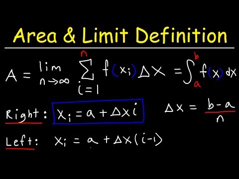 {i_n}\text{,}\) we will assume that \(\lambda_i>\lambda_i+1\text{.}\)
The decreasing list representation of partitions leads us to a handy way to visualize partitions. Given a decreasing list \((\lambda_1,\lambda_2,\ldots \lambda_n)\text{,}\) we draw a figure made up of rows of dots that has \(\lambda_1\) equally spaced dots in the first row, \(\lambda_2\) equally spaced dots in the second row, starting out right below the beginning of the first row and so on. Equivalently, instead of dots, we may use identical squares, drawn so that a square touches each one to its immediate right or immediately below it along an edge. See Figure 3.1.3 for examples. The figure we draw with dots is called the Ferrers diagram of the partition; sometimes the figure with squares is also called a Ferrers diagram; sometimes it is called a Young diagram. At this stage it is irrelevant which name we choose and which kind of figure we draw; in more advanced work the squares are handy because we can put things like numbers or variables into them. From now on we will use squares and call the diagrams Young diagrams.
Figure3.1.3The Ferrers and Young diagrams of the partition (5,3,3,2)
Activity214
Just for practice, draw all the Young diagrams for the partitions of 4 and 5.
With the binomial coefficients, with Stirling numbers of the second kind, and with the Lah numbers, we were able to find a recurrence by asking what happens to our subset, partition, or broken permutation of a set \(S\) of numbers if we remove the largest element of \(S\text{.}\) Thus it is natural to look for a recurrence to count the number of partitions of \(k\) into \(n\) parts by doing something similar. Unfortunately, since we are counting distributions in which all the objects are identical, there is no way for us to identify a largest element. However if we think geometrically, we can ask what we could remove from a Young diagram to get a Young diagram. Two natural ways to get a partition of a smaller integer from a partition of \(n\) would be to remove the top row of the Young diagram of the partition and to remove the left column of the Young diagram of the partition. These two operations correspond to removing the largest part from the partition and to subtracting 1 from each part of the partition respectively. Even though these have some sort of geometric symmetry, the two operations are not symmetric with respect to the number of parts. Thus one might be much more useful than the other for finding a recurrence for the number of partitions of \(k\) into \(n\) parts.
Activity215
In this problem we will study the two operations and see which one seems more useful for getting a recurrence for \(p_n(k)\text{.}\)
(a)
How many parts does the remaining partition have when we remove the largest part (more precisely, we reduce its multiplicity by one) from a partition of \(k\) into \(n\) parts? What can you say about the number of parts of the remaining partition if we remove one from each part?
Hint
These two operations do rather different things to the number of parts, and you can describe exactly what only one of the operations does. Think about the Young diagram.
(b)
If we remove the largest part from a partition, what can we say about the integer that is being partitioned by the remaining parts of the partition? If we remove one from each part of a partition of \(k\) into \(n\) parts, what integer is being partitioned by the remaining parts? (Another way to describe this is that we remove the first column from the Young diagram of the partition.)
Hint
Think about the Young diagram. In only one of the two cases can you give an exact answer to the question.
(c)
The last two questions are designed to get you thinking about how we can get a bijection between the set of partitions of \(k\) into \(n\) parts and some other set of partitions that are partitions of a smaller number. These questions describe two different strategies for getting that set of partitions of a smaller number or of smaller numbers. Each strategy leads to a bijection between partitions of \(k\) into \(n\) parts and a set of partitions of a smaller number or numbers. For each strategy, use the answers to the last two questions to find and describe this set of partitions into a smaller number and a bijection between partitions of \(k\) into \(n\) parts and partitions of the smaller integer or integers into appropriate numbers of parts. (In one case the set of partitions and bijection are relatively straightforward to describe and in the other case not so easy.)
Hint
Here the harder part requires that, after removal, you consider a range of possible numbers being partitioned and that you give an upper bound on the part size. However it lets you describe the number of parts exactly.
(d)
Find a recurrence (which need not have just two terms on the right hand side) that describes how to compute \(p_n(k)\) in terms of the number of partitions of smaller integers into a smaller number of parts.
Hint
One of the two sets of partitions of smaller numbers from the previous part is more amenable to finding a recurrence than the other. The resulting recurrence does not have just two terms though.
(e)
What is \(p_1(k)\) for a positive integer \(k\text{?}\)
(f)
What is \(p_k(k)\) for a positive integer \(k\text{?}\)
(g)
Use your recurrence to compute a table with the values of \(p_n(k)\) for values of \(k\) between 1 and 7.
(h)
What would you want to fill into row 0 and column 0 of your table in order to make it consistent with your recurrence. What does this say \(p_0(0)\) should be? We usually define a sum with no terms in it to be zero. Is that consistent with the way the recurrence says we should define \(p_0(0)\text{?}\)
Hint
If there is a sum equal to zero, there may very well be a partition of zero.
It is remarkable that there is no known formula for \(p_n(k)\text{,}\) nor is there one for \(p(k)\text{.}\) We have seen some ways to compute values of \(p_n(k)\text{.}\) In Section 3.6 we will see more methods to compute values and find properties of these numbers even without ever knowing a formula for them. n p_k(n).
$$
Now consider the partitions of $n$ into $k$ parts. Some of these partitions
contain no 1s, like $3+3+4+6$, a partition of 16 into 4
parts. Subtracting 1 from each part, we get a partition of $n-k$ into
$k$ parts; for the example, this is $2+2+3+5$. The remaining
partitions of $n$ into $k$ parts contain a 1. If we remove the 1, we
are left with a partition of $n-1$ into $k-1$ parts. This gives us a
1–1 correspondence between the partitions of $n$ into $k$ parts, and
the partitions of $n-k$ into $k$ parts together with the partitions of
$n-1$ into $k-1$ parts, so $p_k(n)=p_k(n-k)+p_{k-1}(n-1)$.
Using this
recurrence we can build a triangle containing the $p_k(n)$, and the row
sums of this triangle give the partition numbers. For all $n$,
$p_1(n)=1$, which gives the first column of the triangle, after which
the recurrence applies. Also, note that $p_k(n)=0$ when $k>n$ and we
let $p_k(0)=0$; these are needed in some cases to compute the
$p_k(n-k)$ term of the recurrence. Here are the first few rows of the
triangle; at the left are the row numbers, and at the right are the
row sums, that is, the
partition numbers. For the last row,
each entry is the sum of the like-colored numbers in the previous
rows. Note that beginning with $p_4(7)=3$ in the last row,
$p_k(7)=p_{k-1}(6)$, as $p_k(7-k)=0$.
$$\matrix{
1 & 1& & & & & \color{purple}0& & 1\cr
2 & 1& 1& & & \color{orange}0& & & 2\cr
3 & 1& 1& 1& \color{blue}0& & & & 3\cr
4 & 1& 2& \color{green}1& 1& & & & 5\cr
5 & 1& \color{red}2& 2& 1& 1& & & 7\cr
6 & \color{red}1& \color{green}3& \color{blue}3& \color{orange}2& \color{purple}1& \color{fuchsia}1& & 11\cr
7 & 1& \color{red}3& \color{green}4& \color{blue}3& \color{orange}2& \color{purple}1& \color{fuchsia}1& 15\cr
}$$
Yet another sometimes useful way to think of a partition is with a
Ferrers diagram. Each integer in the
partition is represented by a row of dots, and the rows are ordered
from longest on the top to shortest at the bottom. For example,
the partition $3+3+4+5$ would be represented by
The conjugate of a partition is the one corresponding to the Ferrers
diagram produced by flipping the diagram for the original partition
across the main diagonal, thus turning rows into columns and vice
versa. For the diagram above, the conjugate is
with corresponding partition $1 + 2+4+4+4$. This concept can
occasionally make facts about partitions easier to see than
otherwise. Here is a classic example: the number of partitions of $n$
with largest part $k$ is the same as the number of partitions into $k$
parts, $p_k(n)$. The action of conjugation takes every partition of
one type into a partition of the other: the conjugate of a partition
into $k$ parts is a partition with largest part $k$ and vice
versa. This establishes a 1–1 correspondence between partitions into
$k$ parts and partitions with largest part $k$. n$ is
n$ is
the number of partitions of $n$ into $k$ parts.
Ex 3.3.6
Complete row 8 of the table for the $p_k(n)$, and verify
that the row sum is 22, as we saw in example 3.3.3.
Ex 3.3.7
A partition of $n$ is self-conjugate
if its Ferrers diagram is symmetric around the main diagonal, so that
its conjugate is itself. Show that the number of self-conjugate
partitions of $n$ is equal to the number of partitions of $n$ into
distinct odd parts.
Partitioning Shapes | Definition, Examples, Area, Volume, Measuring
Introduction
In composing shapes, we know that the different shapes of Geometry are squares and rectangles, circles and triangles, trapezoids, rhombuses, stars, hexagons, octagons, and ovals. By making the partition of given shapes we can make a Partitioning shape. Now we are discussing partitioning shapes, which means we are making the partition of given shapes into different small shapes from large shapes. If we have a partitioned shape that consists of a circle and two rectangles, we can make a partition of this shape to get different geometric shapes. For example, we can make a circle from a composite shape by partitioning it into a rectangle and a circle. For this, we can easily break out kite into a circle shape then the shape that we will get from a kite which is a complex will produce a partitioning shape circle. Partitioning shapes are those shapes that are partitioned from composite shapes to two or more geometric shapes. It may refer to any geometric shapes that can be sorted out to break into more than one composite shape that exists in Geometry. Some examples of Partitioning shapes to form the shapes are square and triangle, triangles and circles, etc. Let’s learn about partitioning shapes in detail in this section.
Definition
A shape that can be broken out into more than one of shapes like circles, squares, triangles, stars, ovals, etc, is said to be a decomposite shape or partitioning shape.
The partition shape is a shape in which complex shapes break into a required shape that will be a Unique and defined shape as well. These shapes can be made up by decomposition of Composite shapes
like rectangles, kites, cones, etc. A partition shape is made up by breaking the composite shape into different shapes.
Let us learn about partitioning shapes and how they can be determined.
For example,
Below are some shapes that represent the concept of Partitioning shapes.
We can see that in shape 1 if we break out the shape into two pieces we will get one rectangle and one square. It means that we are doing the partition of shapes into two geometrical shapes rectangle and square.
For shape 2, which is a complex shape because we can break out the given shape into two different shapes in rectangle and triangle by partition.
For shape 3, if we break out the shape that is star into pieces we will get two triangles. It means that we are doing partition of shape into of shapes into two triangles.
For shape 4, if we break out the shape into pieces we will get two right triangles and one rectangle. It means that we are doing partition of shapes into of shapes circles and square.
Area of Partitioning Shapes
The area of Partitioning shapes is a partition of basic geometric shapes like circles, squares, triangles, stars, ovals, etc. To make a partition of any given shape, we must know to calculate the area of some basic shapes like squares, triangles, rectangles, ovals, etc. Let’s learn more about the area of Partitioning shapes through the example
For example,
Make the partition of a given shape and find the area of these partitioning shapes separately?
Solution :
By partition, we will break out the given shape into different geometric shapes. For this, we draw a line to make the partition of the given shape into different shapes. So, we have
Now we have two rectangles. We will find the area of each rectangle by multiplying length and width
For rectangle A,
We have a length is 9 yards and a width is 6 yards
Area of Rectangle A=length ×width
Area of Rectangle A= 9 × 6
Area of Rectangle A = 54 yd2
Now for rectangle B,
We have a length is 6 yards and width is 8 yards
Area of Rectangle B=length ×width
Area of Rectangle B= 6 × 8
Area of Rectangle B = 48 yd2
Now, we will find the area of a right triangle C.
We know that area of a right triangle is
Area of right triangle C = $\frac{1}{2}$ × base × height
Area of right triangle C = $\frac{1}{2}$ × 23 × 9
Area of right triangle C = 103.5
Hence, the area of right triangle C is 103.5 yd2.
Result :
We make the partition of the given shape into two rectangles and the right triangle named is as a rectangle, rectangle B and right triangle find their areas separately.
How to measure
We have some steps to find the area of a partitioning shape
1: Make the Partition of a given shape into different geometric shapes.
2: Find the area of every partitioned geometric shape separately.
3: Write the answer in square units.
For example,
Make the partition of a given shape and find their areas separately?
Solution :
Given shape is a complex shape, we have to make the partition of a given shape.
For this, we will break out the given shape into two right triangles and one square equally. The square has two equal sides of 4 cm length and two right triangles with a 4 cm base and 5 cm hypotenuse of 5cm each.
We have two right triangles, right triangle A and right triangle B.
Now, we will find the area of right triangle A.
We know that area of a right triangle is
Area of right triangle A = $\frac{1}{2}$ × base × height
Area of right triangle A = $\frac{1}{2}$ × 4 × 5
Area of right triangle A = 10
Hence, the area of right triangle A is 10 cm2.
Next, we will find the area of right triangle B.
We know that area of a right triangle is
Area of right triangle B = $\frac{1}{2}$ × base × height
Area of right triangle B = $\frac{1}{2}$ × 4 × 5
Area of right triangle B = 10
Hence, the area of right triangle B is 10 cm2.
Lastly, we have to find the area of square C.
we have four sides and these sides are equal because the shape is square.
So the area of square= (sides )²
Put the any sides in the above formula
The area of square C = (4)2
The area of square C = 16 cm2
Hence, the area of square C is 16 cm2.
Result :
We make the partition of the given shape into two right triangle named right triangle A, right triangle B, and square C also find their areas separately.
Volume of Partitioning Shapes
To find the volume of Partitioning shapes, we need to identify the different shapes that are made from partition. This partition allows working out the volume of each partition shape independently. For composite prisms, where the bases are a composite shape, the area of the bases is the sum of the areas of the partition shape that it is made of. The volume of the prism is then given by multiplying the base area by the height of the prism.
Let’s learn about the volume of Partitioning shapes through some examples.
For example,
Make the partition of a given shape and find their volumes separately?
Solution :
Given shape is rectangular prism and we know that formula for the volume of a rectangular prism is:
Volume is the product of length, width, and height
So,
V = l × w × h
( Where l is the length, w is the width and h is the height of the prism )
For partitioning, we will break out the shape into two parts rectangular prisms as large prisms and small prisms.
Now, we will find the volume of each prism. First, we will find the volume of a large prism
We know that from shape length is 15 inches, width is 4 inches, and height is 5 inches.
Now by the formula of volume
V = l × w × h
V = 15 × 4 × 5
V = 300
Hence, the volume of the large prism is 300 cubic inches.
Next, we will find the volume of the small prism
We know that from shape length is 11 inches, width is 3 inches, and height is 4 inches.
Now by the formula of volume
V = l × w × h
V = 11 × 3 × 4
V = 132
Hence, the volume of the large prism is 132 cubic inches.
Result :
We make the partition of the given shape into two prisms, large prisms, and small prisms, and find their volumes separately.
How to measure
We have some steps to find the volume of a partitioning shape.
1: Make the partition of the given shape into different geometric shapes.
2: Find the volume of every partitioning geometric shape separately.
3: Write the answer in cube units.
Solved Examples :
Example 1 :
What is the partition of the given shape and the area of the shaded region?
Solution :
The partition of the given shape is two triangles simple A and B. We have to find the area of the shaded region between these partitioning shapes.
To find the area of a figure with a hole in it, subtract the area of triangle A
from the area of triangle B.
Area of a triangle B = $\frac{1}{2}$ x base × height
From the above shape, we know the base and height of triangle B, base and height are 18 km.
Putting the values in the above formula
Area of a triangle B = $\frac{1}{2}$ x 18 × 18
Area of a triangle B = 162 square kilometers
Hence, The area of triangle B is 162 square kilometers.
Next, find the area of triangle A, Base is 31 km and height is 28 km
Area of a triangle A = $\frac{1}{2}$ x base × height
Area of a triangle A = $\frac{1}{2}$ x 31 × 28
Area of a triangle A = 434 square kilometers
Hence, The area of triangle B is 434 square kilometers.
Finally, subtract the triangle Area A from the triangle B to find the area of the shaded region.
The area of the shaded region = Area of triangle A – Area of a triangle B
The area of the shaded region = 434 162
The area of the shaded region = 272
The area of the shaded region is 272 square kilometers.
Result :
We have calculated the Area of all the partition shape i.g Right triangles and find the shaded area between the partitioning shapes.
Example 2 :
What is the partition of a given shape and find the area of every partition shape separately?
Solution :
We will make the partition of the given shape into a right triangle, rectangle , and one semicircle as shown in the figure below
Next, we have to find the area of each partition shape separately.
For this first, we will calculate the area of the Right triangle.
We know that area of the Right triangle is equal to
A = $\frac{1}{2}$ × base × altitude
Putting the values of base and altitude in the above formula, we will get the area of the Right triangle.
A = $\frac{1}{2}$ × 30 × 40
A= 600 cm²
Secondly, we will calculate the area of the Rectangle.
We know that area of the Rectangle is equal to
A = Lenght × width
Putting the values of length and width in the above formula, we will get the area of the Rectangle
A = 60 × 40
A= 2400 cm²
Now, we will calculate the area of the semicircle.
We know that area of the semicircle is equal to
A = 1/2 π × r²
A= 1/2 × 3.1415 × (15)²
A= 353.42 cm²
Result :
We have calculated the Area of all the partition shapes i.g Right triangle, rectangle, and semicircle
Example 3 :
What is the partition of given shapes and find the volume of each partitioning shape separately?
Solution :
For the area of partitioning shape, first, we will make partition of this complex shape into geometric shapes so, we can show that by figure, We have broken out the given complex shape into two rectangles
and one right triangle. Firstly, we will find the area of the Right triangle.
From shape A, we know that base is 6 and 5 in height So,
The area of a right triangle is = 1/2 base × height
Area of shape A= 1/2 × 6 × 5 = 15
Hence, the area of the right triangle is 15 ft²
Secondly, we have rectangle B, for this, we have length 6 and width 9
So the area of rectangle B will be
Area of Rectangle B= 9×6
Area of Rectangle B= 54
Hence, the area of Rectangle B is 54 ft²
Now, we have the last rectangle C, for this, we have length 4 and width 6
So the area of rectangle C will be
Area of Rectangle C= 4×6
Area of Rectangle C= 24
Hence, the area of Rectangle C is 24 ft²
Result:
We make the partition of the given shape into two rectangles A and B and one right triangle also find their volumes separately.
Example 4 :
Find the partition of the given shape then find the volume of each shape that will be obtained by partition?
Solution :
Given shape is rectangular prism and we know that formula for the volume of a rectangular prism is:
Volume is the product of length, width, and height
So,
V = l × w × h
( Where l is the length, w is the width and h is the height of the prism )
To find the volume of a given shape, we will break out the shape into two parts as rectangular prisms.
Now, find we will find the volume of each Prism that is obtained by partition. First, we will find the volume of a large prism
We know that from shape length is 11 centimeters, width is 4 centimeters, and height is 6 centimeters.
Now by formula of volume
V = l × w × h
V = 11 × 4 × 6
V = 264
Hence, the volume of the large prism is 264 cubic centimeters.
Next, we will find the volume of the small prism.
We know that from shape length is 2 centimeters, width is 2 centimeters, and height is 5 centimeters.
Now by formula of volume
V = l × w × h
V = 2 × 2 × 5
V = 20
Hence, the volume of the small prism is 20 cubic centimeters.
Result :
We make the partition of given the shape into two prisms small are large and find their volumes separately.
Example 5 :
For the given shape, we have the Partition of shape into 4 equal squares.
Find the area of the square?
Solution :
We know that a given complex shape by breaking out we have five sides and these sides are equal because the shape is square.
So the area of square= (sides )²
Put the side length in the above formula
The area of square= (4)²
The area of square= 16
Hence, The area of the square is 16 cm2
Example 6 :
What is the partition of a given shape and find the area of shapes that are obtained by the partition of a given shape?
Solution :
By partitioning the shape, we will make the partition of the shape into geometric shapes. For this, we draw a line for the partition of the given shape into different geometric shapes. By Partitioning, we have two rectangles and one triangle. We will find the area of each rectangle by multiplying length and width and the area of the triangle by multiplying base and width.
For rectangle A,
We have length l=4 mm and width w=18 mm
Area of Rectangle A=length ×width
Area of Rectangle A= 4 × 18
Area of Rectangle A = 72 mm2
Now for rectangle B,
We have length l=5 mm and width w=10 mm
Area of Rectangle B=length ×width
Area of Rectangle B= 5 × 10
Area of Rectangle B = 50 mm2
Lastly, we will find the area of the Right triangle.
From shape C, we know that base is 19 and 14 in height.
So,
The area of a right triangle is = 1/2 base × height
Area of shape C= 1/2 × 19 × 14 = 133 mm².
Result :
We make the partition of the given shape into two rectangles A and B and one right triangle also find their areas separately.
Key Facts and Summary
- Partitioning shapes can be broken out by Partitioning into more than one of the shapes like circles, squares, triangles, stars, ovals, etc.
- Area of Partitioning shape is can be calculated by their fixed formulas after partitioning shapes.
- Decomposite shapes Or partitioning shapes are those shapes that are obtained by the partition of some different complex shape into two or more geometric shapes.
- We can measure the area and volume by following steps :
- By making the partition of given shapes into different geometric shapes.
- Finding the area and volume of Partitioning shape separately.
- If the dimensions of all the that are obtained by a partition are raised, the area of Partitioning shapes also increases.
- The area of Partitioning shape changes as it depends on the individual area of a geometric shape that is obtained by making the partition of given shapes which gets changed when the dimensions are increased or raised.
- We have a fixed formula to calculate the area of partitioning shapes.
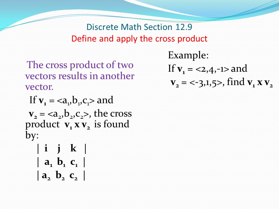
2-D and 3-D Shapes Kindergarten Math Worksheets
Partitioning Shapes 1st Grade Math Worksheets
Shape Partitions (Rectangles and Circles) 2nd Grade Math Worksheets
Browse All Worksheets
We spend a lot of time researching and compiling the information on this site. If you find this useful in your research, please use the tool below to properly link to or reference Helping with Math as the source. We appreciate your support!
|
Feedback COGNITIVE Willpower leads to action, and positive actions form a positive attitude How to determine the range of your voice — your vocals How the target learns about your desires before you take action. How Companies Predict and Manipulate Habits Healing Habit How to get rid of resentment Conflicting views on the qualities inherent in men Self -confidence training The delicious «garlic salad» still life Application. How to learn to take responsibility Why do we need boundaries in relationships with children? Reflective elements on children’s clothing How to beat your age? Eight Unique Ways to Achieve Longevity How to Hear the Voice of God The WHO BMI Classification of Obesity Chapter 3. The Covenant of a Man with a Woman Axes and planes of the human body — The human body consists of certain topographic parts and sections in which organs, muscles, blood vessels, nerves, etc. are located. Wall trimming and jamb cutting — When the house lacks windows and doors, a beautiful high porch is still only in the imagination, you have to climb the stairs from the street into the house.
Second Order Differential Equations (Price Forecast Market Model) — In simple market models, supply and demand are usually assumed to depend only on the current price of the commodity. |
The concept is a form of thinking that reflects the essential (distinctive) properties of the objects of study. A concept is considered correct if it correctly reflects real-life objects. The content of the concept is the set of all essential features of this concept. The scope of the concept is the set of objects to which the concept is applicable. Essential (characteristic) properties are such properties, each of which is necessary, and all together are sufficient to characterize the objects belonging to the concept.
Classification is a sequential, multistage partition of a set into two classes with the help of some property. The correct classification of concepts requires the following conditions: — classification is carried out according to a certain attribute that remains unchanged during the classification process; — the concepts resulting from the classification are mutually independent, that is, none of them should be included in the scope of another class.
— the sum of the volumes of concepts resulting from the classification is equal to the volume of the original concept; — in the process of classification, they move to the closest species in this generic concept. Example of correct classification Types of definitions Definition of a concept is a sentence that reveals the content of a concept, i. Axiomatic (indirect) definitions — definitions of initial concepts which are given by means of initial concepts of some theory through its axioms (for example: concept of area of a figure). In the axiomatic construction of a mathematical theory, some concepts remain undefined (point, line, plane). Descriptions are definitions of mathematical objects by indicating their properties (“The number that, when multiplied by the length of the diameter, gives the length of its circumference” — a description of the number π). Definitions through genus and specific differences — definitions in which the defined is distinguished from the objects of a certain area, which is explicitly mentioned in the definition (genus), by indicating the characteristic property of the defined (specific difference). Genetic definitions. These are definitions that describe or indicate the method of its origin, formation, occurrence, construction. Genetic definitions are a kind of definition through the genus and specific differences. For example: «A sphere is a surface obtained by rotating a semicircle around its diameter.» Inductive definitions are those that allow one to obtain new objects from similar objects (theories) by applying specific operations to them. For example, the definition of a natural number in mathematics is introduced by induction. Definition through abstraction — definitions associated with the selection of objects through the establishment of relations between them of equality, equivalence, identity. In the definition via abstraction, a mathematical concept is defined as a family of equivalence classes with respect to some equivalence relation.
Entrust your work ✍️ to a candidate of sciences! Name We will help with coursework, control, diploma, essay, practice report, research and any other work By clicking the «Continue» button, I accept the privacy policy
|
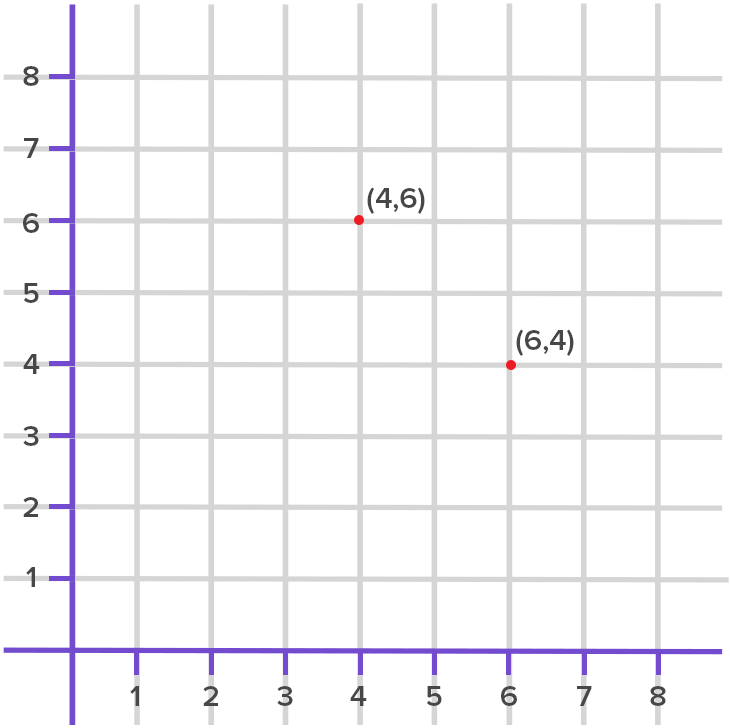 take mummy? Shilajit for hair, face, fractures, bleeding, etc.
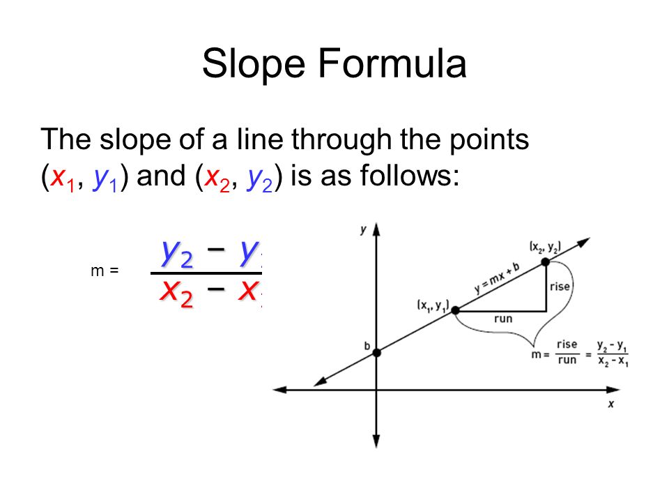
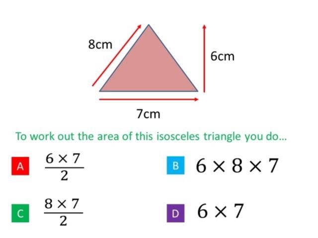
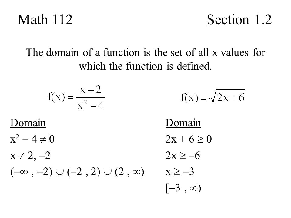 a set of conditions necessary and sufficient to select a class of objects belonging to the concept being defined.
 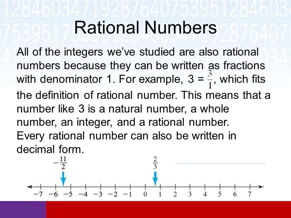 For example: «A square is a rectangle with equal sides.»
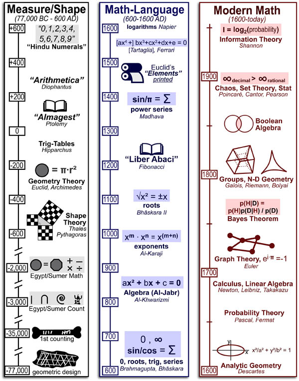
COXTER PARTITION, ROOT SYSTEMS AND THAT WATER
In the article «Life, the water molecule and the golden ratio» [1] (see «Science and Life» No. 10, 2004) a hypothesis was put forward that the melt water molecule «with a high degree of probability has a structure that is as close as possible to the harmonious triangle of the golden ratio with a bond angle close to 108 °, and with a ratio of bond lengths of approximately 0.618-0.619. The authors have no experimental confirmation of this hypothesis, just as there is no theory of its justification.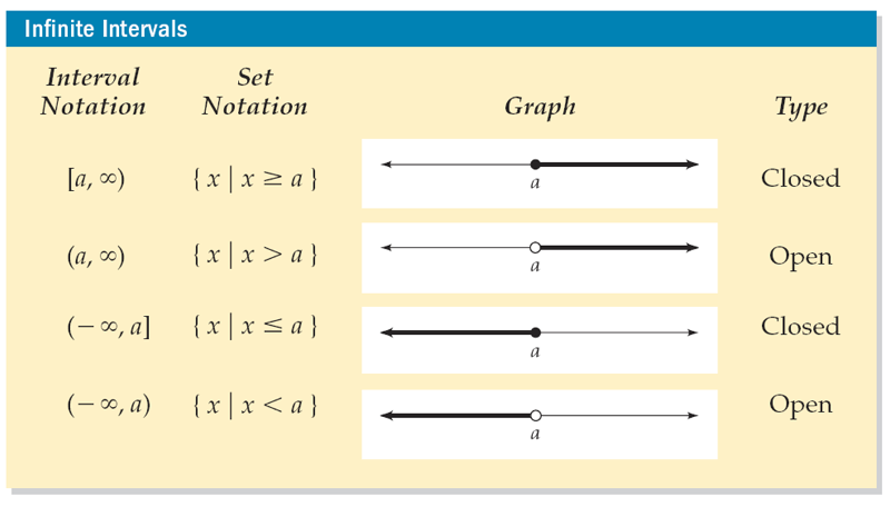 There is only a conjecture expressed on these pages, which can, of course, be disputed. «The authors of this article agree with this assumption, moreover, they believe that melt water is a flat quasicrystal with a Penrose partition. We have a mathematical justification for this hypothesis, popularly In conclusion, we want to agree with the statements of the authors of the articles [1, 2] that joint creativity with students «confirms the creative possibilities of young people and inspires hope that the language of science will not be lost.»
Fig. 1. Model of the melt water molecule.
Fig. 2. Penrose rhombus and the first golden triangle.
Fig. 3. The second Penrose rhombus and the third golden triangle.
Fig. 4a. Partition of a regular hexagon into three Kepler rhombuses.
Fig. 4b. Rhombus Kepler.
Fig. 5. Coxeter decomposition of a regular hexagon.
Fig. 6. Cells of Bravais lattices: an arbitrary parallelogram, a rectangle, an arbitrary rhombus, a square, and a Kepler rhombus.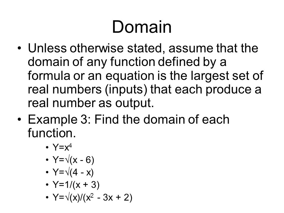
Fig. 7a, 7b. Generalized Coxeter triangles are golden triangles.
Fig. 8. Splitting a pentagon into five golden triangles.
Fig. 9a. Star polygon.
Fig. 9b. Star polygon with completed Penrose rhombus.
‹
›
View full size
What we see —
Bottom visibility only,
True Essence
Things are not visible.
Omar Khayyam
Experimental data on the structure of the water molecule and Penrose tiling
Back in 1810, the English physicist John Dalton built models of some molecules from balls and rods. The balls corresponded to the atoms, the rods to the chemical bonds in the molecule. Of course, at that time Dalton could not indicate the magnitude of the distances between atoms in a molecule and bond angles. This is still difficult, for example, for water in the liquid state. That is why the authors of the article [1] write that they cannot experimentally confirm their hypothesis.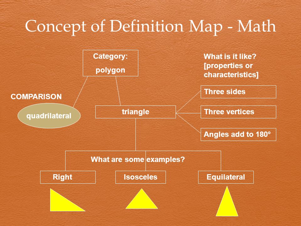 However, if we consider substances in a gaseous or solid state, then the geometric configurations and parameters of the molecules can be determined. Relevant data are available in reference books, for example, in the book by N. G. Rombidi and S. M. Tolmacheva «Tables of standard and reference data. Geometric configuration and internuclear distances of molecules and ions in a gaseous medium.» The book came out at 1978 at the Standards Publishing House.
Using reference data of this kind and extrapolating them, the authors of [1] arrive at a model of the melt water molecule shown in Fig. 1.
The figure shows the values of internuclear distances (they are obviously the same) and the value of the HOH bond angle. Further connecting the vertices of HH and attaching another similar triangle symmetrically to the resulting triangle, we get one of the two famous Penrose rhombuses (Fig. 2).
The figure shows a Penrose rhombus with interior angles of 108° and 72°, divided by a diagonal into two equal triangles. If we take that side HH = 1, then, as shown in [1], we get a triangle HH , in which
Such a triangle in the article [2] is called the first triangle of the golden ratio. For brevity, we will call it the first golden triangle.
On fig. 3 shows another Penrose rhombus with internal angles of 144 and 36°. Note that
(vertex angle B is obtuse and its cosine is negative). As already noted,
but now the 36° angle is the angle at the base of the golden triangle.
The authors of [2] introduce another golden triangle with angles of 54° at the base and 72° at the apex. The first triangle is obtained by cutting the rhombus in Fig. 3 diagonal ВD , and the second — if you cut the rhombus in fig. 2 diagonal OB . We will talk about these triangles below, but for now, we note that in the late 1970s, Penrose [3] developed an algorithm for partitioning a plane without voids and overlaps by the two types of rhombuses indicated, and even patented several samples of room wallpaper and their partitions into rhombuses. The Penrose tiling is not periodic, but any finite piece occurs in it an infinite number of times and necessarily appears in a circle of sufficiently large radius with any center on the plane. In addition, this partition transforms into itself when rotated through angles that are multiples of 72°. A few years after the discovery of Penrose, at 19In the 1980s, new types of two-dimensional and three-dimensional materials were discovered, called quasicrystals, whose atoms are located at the vertices of rhombuses that form a Penrose tiling. Later, physicists found quasicrystals with symmetry axes of the eighth, tenth and twelfth orders. After the discovery of quasicrystals, partitions of three-dimensional space into prisms were considered, the bases of which were Penrose rhombuses.
Let us now recall another story, seemingly unrelated to the previous one.
Even before Penrose’s discovery, the American architect Richard Buckminster Fuller in 1942 (!) created a geodesic dome — a sphere formed by a lattice of polygonal elements.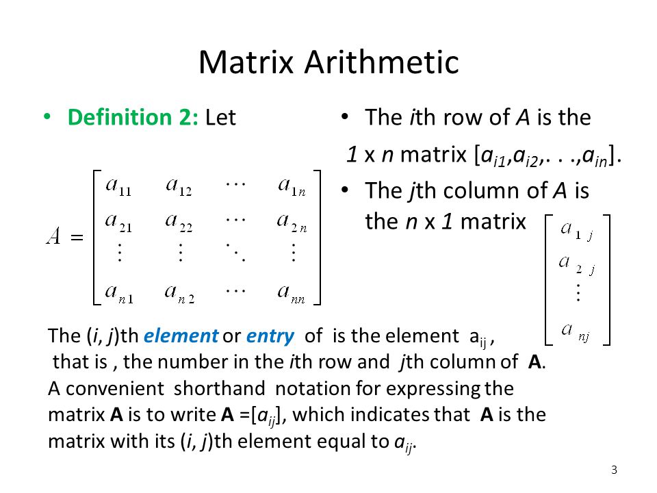 A fascinating story about this invention can be read in Alexander Leizerovich’s article «Mark Fuller», published in 2004 in the journal «Knowledge is Power». Two years after Fuller’s death, in 1985, molecules of a spheroidal structure were discovered, formed by polygons with carbon atoms at the vertices (see «Science and Life» No. 7, 1992). In honor of Fuller, they were called fullerenes, and the molecular crystals consisting of them were called fullerites (see «Science and Life» No. 10, 1995). Projecting a fullerite crystal onto a plane in a certain way (we do not specify here), we obtain a Penrose tiling of the plane, if we assume that, as is customary in crystallography, this crystal is infinite.
The article by V. S. Belyanin and E. N. Romanova [2] deals with the Penrose tiling and the connection between Penrose rhombuses and golden triangles. Therefore, in their next article, a hypothesis is expressed about the structure of the melt water molecule. Knowing that liquid crystals exist, it is natural to add one more hypothesis to this hypothesis: melt water is nothing but a liquid flat quasicrystal.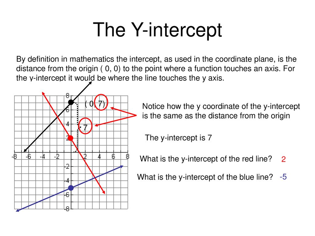 Let’s try to prove it mathematically.
Coxeter tiling,
crystals and quasi-crystals
If quasicrystals are associated with Penrose tilings, then crystals are associated with the so-called Coxeter tilings. Before giving their definition, let us turn to the general definition of partitioning a space into polyhedra, since it is not found in [1, 2].
Definition 1 . A partition of a space into convex polyhedra is such a filling of it with polyhedra, in which each point of the space belongs to some polyhedron and no two polyhedra of the partition have a common interior point. Here we will consider partitions of space and polyhedra into polyhedra of a special kind — Coxeter polyhedra.
Definition 2 . A convex polytope Р is called a Coxeter polytope if all its dihedral angles are equal
, where n is a natural number, n 2.
A flat polyhedron is a polygon, and its angles play the role of dihedral angles, therefore all angles of a Coxeter polygon are either right or acute
, where n > 2.
Examples of Coxeter polygons: a square (its angles are
equilateral triangle (its angles are
and others.
Definition 3(4). The Coxeter partition of the space X (a convex polyhedron R ) is its partition into Coxeter polyhedra (into a finite number of Coxeter polyhedra), in which polyhedra having a common face are symmetric with respect to this face.
The definition of a Coxeter tiling of a convex polyhedron is given in parentheses. P , which appeared quite recently in the works of A. A. Felikson (see, for example, [4]).
Let us give examples of the Coxeter tiling of the plane and plane polygons.
The first example was actually given several hundred years ago by the famous German astronomer and mathematician J. Kepler. In 1611 (!) his book «New Year’s Gift, or About Hexagonal Snowflakes» appeared. It was one of the first, if not the very first piece of non-fiction literature on mathematics.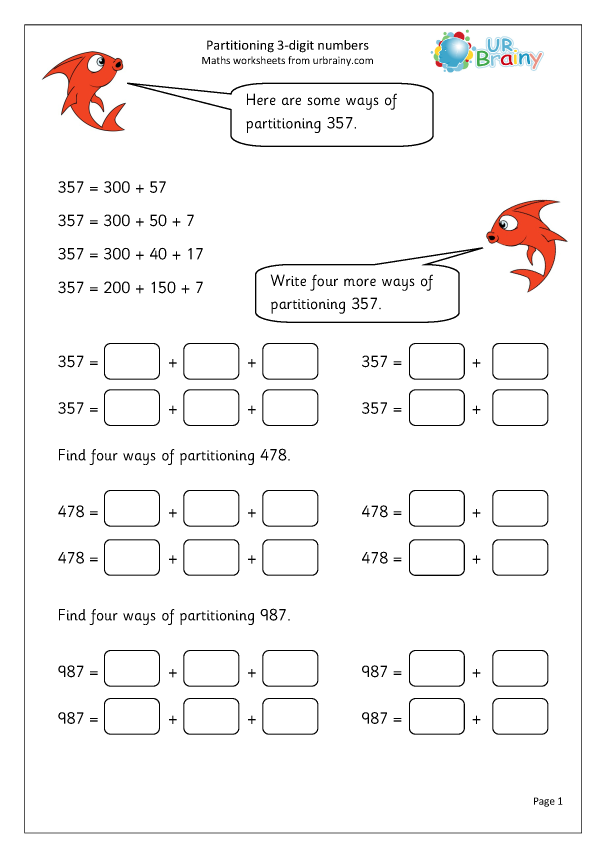 Kepler writes: «Since whenever it starts to snow, the first snowflakes are in the shape of a hexagonal star, there must be a certain reason for this, for if this is an accident, then why are there no pentagonal or heptagonal snowflakes?»
Next, Kepler considers the partition of the plane into regular hexagons and shows that there can be no gaps with such a cover, in contrast to a pentagonal cover. In the latter case, as Kepler notes, cracks will appear through which, for example, cold will penetrate to the bees in the hive through the honeycombs.
It is easy to pass from the partitioning of the plane by hexagons to its partitioning by rhombuses with internal angles of 120 and 60°. For this, a regular hexagon is divided into three rhombuses, as shown in Fig. 4a.
Kepler considered just such rhombuses, so we will call them Kepler’s rhombuses (because there are also Bravais and Penrose rhombuses).
The brilliant Kepler foresaw the important role that diamond-shaped bodies would play in space.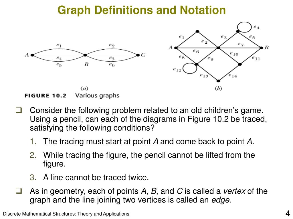 He wrote: «All space can be filled with regular rhombic solids so that the same point will serve as the vertices of four spatial angles with three edges, as well as six spatial angles with four edges.»
Let’s return to Kepler’s flat rhombuses. The rhombus shown in Fig. 4b can be divided into two regular Coxeter triangles by drawing its diagonal through an angle of 120°.
It follows that a regular hexagon can be divided into six regular Coxeter triangles (Fig. 5).
In the work of A. A. Felikson [4], polyhedra that admit a Coxeter partition are called quasi-Coxeter ones. From all such partitions of finite figures we can pass to partitions of the whole plane.
The vertices of the partition polygons form a lattice. If we imagine that there are atoms at the vertices of such a lattice, then we will get a model of a crystal.
Back in 1848, the former brave sailor O. Brave listed all types of lattices in the plane and in space that have irregular symmetries.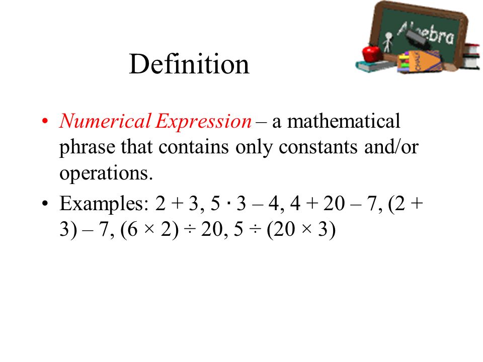 So, on the plane there are five types of lattices: general, rectangular, rhombic, square and hexagonal. The polygons that subdivide the entire plane are shown in Fig. 6.
Note that the square and rectangle are Coxeter polygons since their angles are
In addition to them, Coxeter triangles are triangles with angles 90, 45 and 45°, into which a square and an isosceles right triangle are divided, and with angles of 30, 60 and 90°, into which a right triangle with an aspect ratio of 1 : 2 is divided. All modern crystallography is based on such partitions.
The reader may have a question: «Why is it impossible to consider partitions of the plane (and space) into polygons (polyhedra) of different types?». Penrose was one of the first to consider such partitions. In this connection, and in connection with the theory developed by A. Felikson, the question arises of generalizing the concept of a Coxeter partition. And we come to the next definition.
Definition 4. A generalized Coxeter polygon is a polygon whose angles are equal to rational parts of the form
p and q are natural numbers. If p = 1, we get the usual Coxeter polygons. If p > 1, then the golden triangles shown in fig. 7a and 7b. Indeed,
(question: are there other generalized Coxeter triangles?).
It is now natural to generalize the definition of a Coxeter tiling of a plane and a polygon. It is so simple that we do not even present it here. In Definition 3, instead of the words «Coxeter polygon» one should write «generalized Coxeter polygon». From the above drawings of Penrose rhombuses, it immediately follows that they can be partitioned into generalized Coxeter triangles — golden triangles. And since the whole plane can be divided into two types of Penrose rhombuses, there is a partition of the plane into golden generalized triangles of two types, shown in Fig. 7a and 7b.
Finally, let’s see how water molecules can form a quasi-crystal. As Kepler already noted, snowflakes cannot have a regular pentagonal shape, since regular pentagons cannot divide a plane. However, the regular pentagon itself can be divided into five golden triangles with angles of 72° at the top and 54° at the base.
In the spirit of [4], the pentagon in Fig. 8 can be called generalized quasi-Coxeter. The angles at the vertices of a regular pentagon are 108°, but the parallelogram is ABCO (and AODE ) has interior angles of 108 and 54° and is not a Penrose diamond (it is not a diamond at all). But the Penrose diamonds appear! To get them, we add to the golden triangles into which our pentagon is divided, symmetrically the same triangles, as shown in Fig. 9a.
Shown in fig. 9a shows a stellated pentagon that can be partitioned into golden triangles with angles of 54, 54 and 72° (there are 10 of them) and into five Penrose rhombuses with interior angles of 108 and 72°.
Interestingly, Kepler also considered stellated polyhedra! The most famous of them, translated from Latin, was called «morning star».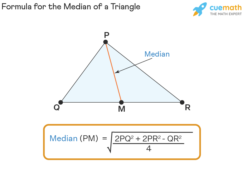 We see from this example that when considering partitions, it is not necessary to consider, as is usually done, convex polyhedra.
Here the reader may have a question: «And where is the second Penrose rhombus with internal angles of 144 and 36 °?». Let’s calculate by looking at Fig. 9a, the sum of all the angles of the golden triangles, for example, at the vertex B . It is equal to 4 . 54 = 216°, since four golden triangles converge at the top. Therefore, the remaining angle at the vertex B is equal to . Adding a Penrose rhombus with interior angles of 144 and 36°, as shown in Fig. 9b, we will fill the gap between the rays of the star and at the vertex B , and at the other vertices. There is another 36° angle here. This is the central angle of a regular decagon, since
This decagon breaks into golden triangles with 72° base angles and 36° apex angles. So we get an algorithm for partitioning the plane into golden triangles of two types, Penrose rhombuses of two types. Therefore, it can be assumed that two-dimensional liquid quasi-crystals, like snowflakes, are formed according to this algorithm of nature itself. This assumption is even more confirmed if we introduce into consideration the internal symmetry that crystals and quasicrystals possess.
Using Coxeter partitions and other apparatus of modern mathematics, it will be possible to study the symmetry of two-dimensional (flat) crystals and quasicrystals, and when entering three-dimensional space, the symmetry of fullerenes and fullerites.
Literature
1. Belyanin V. S., Romanova E. N. Life, the water molecule and the golden ratio // Science and Life, 2004, No. 10.
2. Belyanin V. S., Romanova E. N. Golden proportion. New look // Science and life, 2003, No. 6.
3. Penrose R. Pentaplexity // Evreka, 1978, V. 39, p. 16-22.
4. A. A. Felikson, “Coxeter tilings of bounded hyperbolic pyramids and triangular prisms,” Mathematicheskie Zametki, No.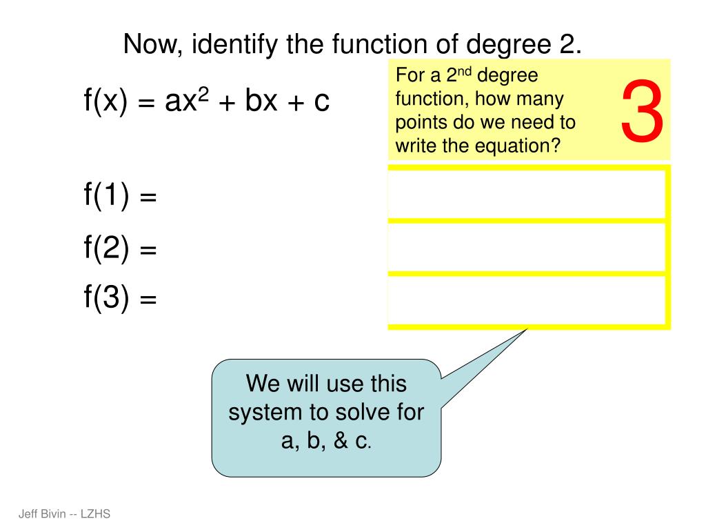 4, 2004.
Circulation 100,000 copies.
Series Library «Quantum», issue 7
|
|||||||||||
The book is an introduction to elementary algebra and group theory, which is widely used in modern mathematics and physics, crystallography, solid state physics and elementary particle physics. All introduced concepts are explained in detail using simple geometric examples. The book includes an addition written by Yu.P.Soloviev. For pupils, teachers, students.
Contents
PREFACE.
INTRODUCTION.
Chapter I. THE CONCEPT OF A GROUP.
§ 1. The simplest concepts of set theory.
1.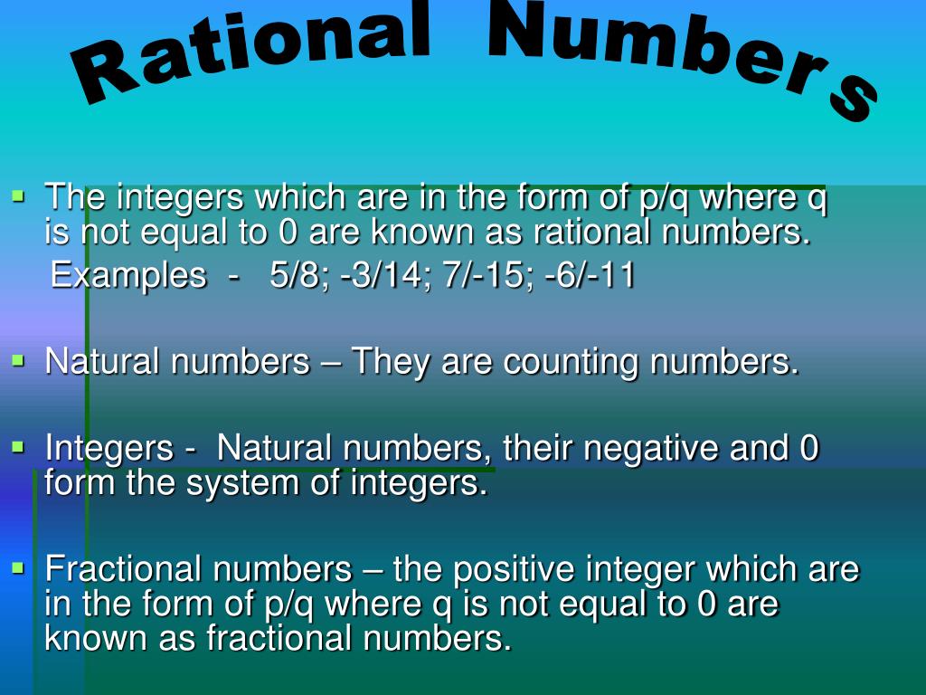 The sum of sets.
2. Intersection of sets.
3. Displays or functions.
4. Splitting a set into subsets.
§ 2. Introductory examples.
1. Operations on integers.
2. Actions on rational numbers.
3. Rotations of an equilateral triangle.
4. Klein group of the fourth order.
5. Turns of a square.
§ 3. Definition of a group.
§ 4. The simplest theorems about groups.
1. The product of any finite number of elements of a group.
The first rule for opening parentheses.
2. Neutral element.
3. Inverse element.
4. Remarks on group axioms.
5. «Multiplicative» and
«additive» terminology in group theory.
Chapter II. GROUPS OF SUBSTITUTIONS.
§ 1. Definition of permutation groups.
§ 2. The concept of a subgroup.
1. Examples and definition.
2. Condition for a subset of a group to be a subgroup.
§ 3.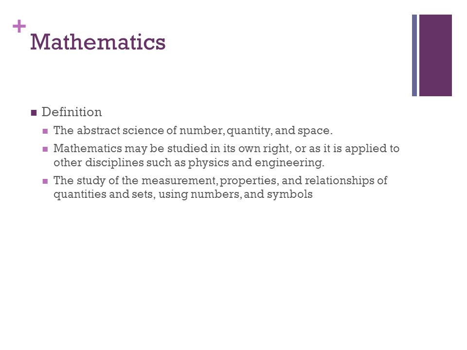 Substitutions as mappings of a finite set
to myself. Even and odd substitutions.
1. Substitutions as mappings.
2. Even and odd substitutions.
Chapter III. ISOMORPHOUS GROUPS. Cayley’s theorem.
§ 1. Isomorphic groups.
§ 2. Cayley’s theorem.
Chapter IV. CYCLIC GROUPS.
§ 1. A subgroup generated by a given element of a given
groups. Definition of a cyclic group.
§ 2. Finite and infinite cyclic groups.
§ 3. Systems of generators.
Chapter V. SIMPLE SELF-COMBINING GROUPS.
§ 1. Examples and definition of the self-combination group
geometric shapes.
1. Self-matching of regular
polygons in their plane.
2. Self-alignment correct
polygon in 3D space.
3. General definition of a group
self-combinations of a given figure in space or on a plane.
§ 2. Self-coincidence groups of a line and a circle.
§ 3. Groups of rotations of regular pyramid and double
pyramids.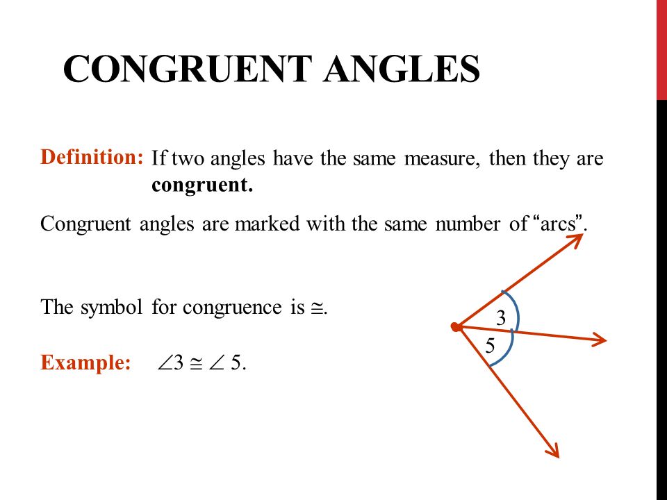
1. Pyramid.
2. Double pyramid (dihedron).
3. The case of degeneracy: groups
turns of a segment and a rhombus.
§ 4. Group of rotations of a regular tetrahedron.
§ 5. Group of rotations of a cube and an octahedron.
§ 6. Rotation group of icosahedron and dodecahedron. General remark
on rotation groups of regular polyhedra.
Chapter VI. INVARIANT SUBGROUPS.
§ 1. Conjugate elements and subgroups.
1. Transformation of one element
groups with the help of another.
2. An example of a tetrahedron group.
3. Conjugated elements.
4. Subgroup transformation.
5. Examples.
§ 2. Invariant subgroups (normal divisors).
1. Definition.
2. Examples.
Chapter VII. HOMOMORPHOUS MAPPINGS.
§ 1. Definition of a homomorphic mapping and its kernel.
§ 2. Examples of homomorphic mappings.
Chapter VIII. DIVISION OF A GROUP INTO CLASSES
FOR THIS SUBGROUP. FACTOR GROUP.
§ 1. Left and right classes.
1. Left-sided classes.
2. The case of a finite group G.
3. Right hand classes.
4. Coincidence of right-hand classes with
left-sided in the case of invariant subgroups.
5. Examples.
§ 2. Factor group by a given invariant subgroup.
1. Definition.
2. The theorem on homomorphic
mappings.
Addendum. GROUPS OF MOVEMENTS OF THE PLANE AND SPACE
AND THEIR SUBGROUPS. (Yu.P. Soloviev.)
1. Group of displacements of the plane.
2. Group of space displacements.
3. End subgroups of the movement group
space.
|
|||||||||||
Permanent address of this page:
http://math.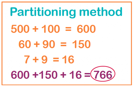 ru/lib/bmkvant/7
Mathematical analysis. Part 4 | Open video lectures of MSU training courses
List of all lecture topics
Lecture 1. Multiple Riemann integral. Basic definitions.
Multiple Riemann integral
Beam definition
Beam split assertion
Determining the scale of the split
Integral sum
Definition of the multiple Riemann integral
A necessary condition for integrability
Examples of Integrable Functions
Properties of multiple integrals
Theorem on passage to the limit under the integral sign
Lecture 2. The theorem on passage to the limit under the integral sign.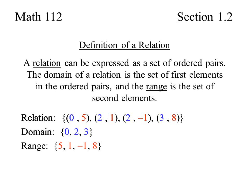
Proof of the theorem on passage to the limit under the integral sign
Assertion on the integrability of a continuous function
An example of a function that cannot be reduced to a step function
Theorem on monotonic approximation by step functions
Fubini’s theorem
Lecture 3. Fubini’s theorem.
Reminder of the previous lecture
Proof of Fubini’s theorem
Integration by parts formula
Reminder of the integrability criterion
Definition of a set of measure zero according to Lebesgue for a multidimensional integral
Examples of sets of measure zero
Zero subset assertion
Lebesgue criterion
Lecture 4.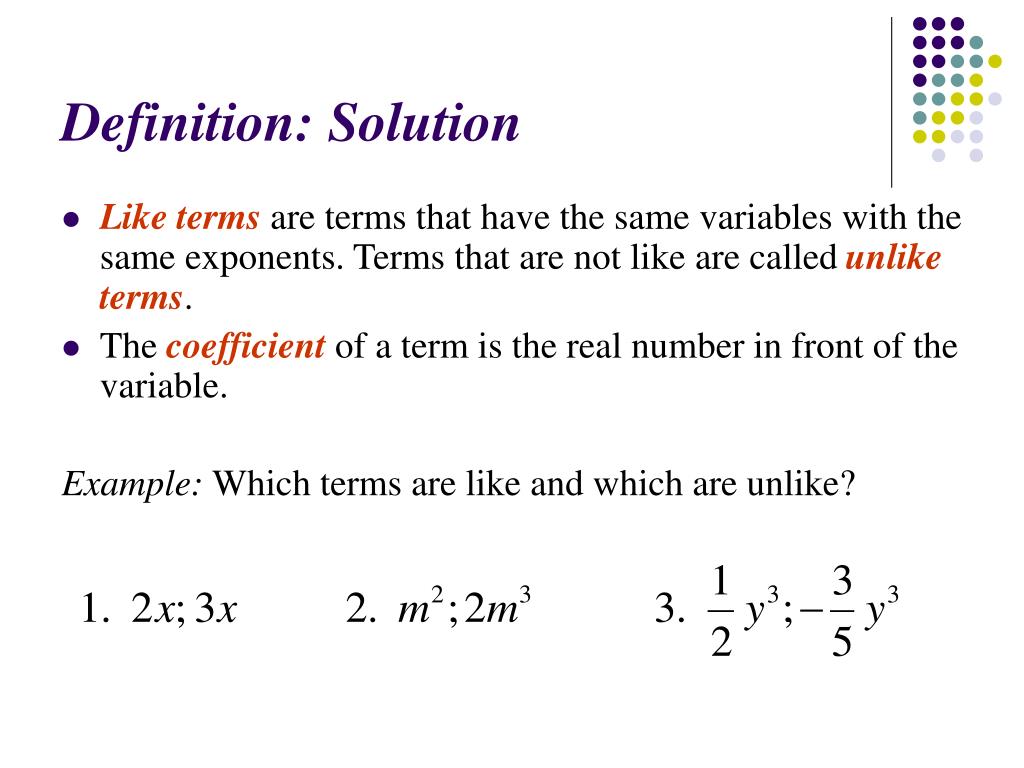 Set integral and Jordan measure.
Reminder of the last lecture
Proof of the Lebesgue criterion
Definition of an integral over a set
An example of integrable set indicators
Definition of the Jordan measure
Lebesgue criterion for admissible sets
Lecture 5. Admissible sets and properties of the integral on them.
Reminder of the last lecture
Properties of the integral over admissible sets
Fubini’s theorem
Variable Change Formula in Multiple Integral
Lecture 6. Variable change formula.
Reminder of the last lecture
Continuation of the proof of the formula for the change of variables in a multiple integral
Lecture 7.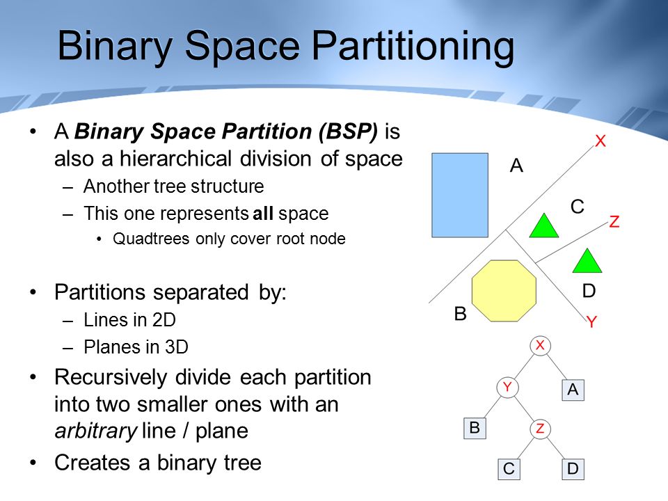 Brouwer’s theorem.
Continuation of the proof of the formula for the change of variables in a multiple integral
Repetition of the proof scheme
Linear transformation problem
Consequence from the variable change formula
Brouwer’s theorem
Lecture 8. Drum lemma and hedgehog theorem.
Proof of Brouwer’s theorem
Drum Lemma
Corollary from Brouwer’s theorem
Theorem on the existence of a singular point on the sphere
Lecture 9. Riemann’s multidimensional improper integral.
Multidimensional Improper Riemann Integral
Exhaustion choice theorem
An example of applying the theorem
Convergence sign
Lecture 10. Measure and integral over measure.
Reminder of facts about the multidimensional Riemann integral
Measure and integral over measure
Definition of Algebra and Sigma Algebra
Borel sigma algebra
Measure definition
Construction of Carathéodory
Outer measure theorem
Lecture 11. Lebesgue measure and its applications.
Reminder of the last lecture
Lebesgue measure
Relationship between volume and Lebesgue measure
Lecture 12. Hausdorff measure.
Reminder of the last lecture
Hausdorff measure
Assertion on the external Hausdorff measure
Coincidence of the Hausdorff measure and the Lebesgue measure
Lecture 13.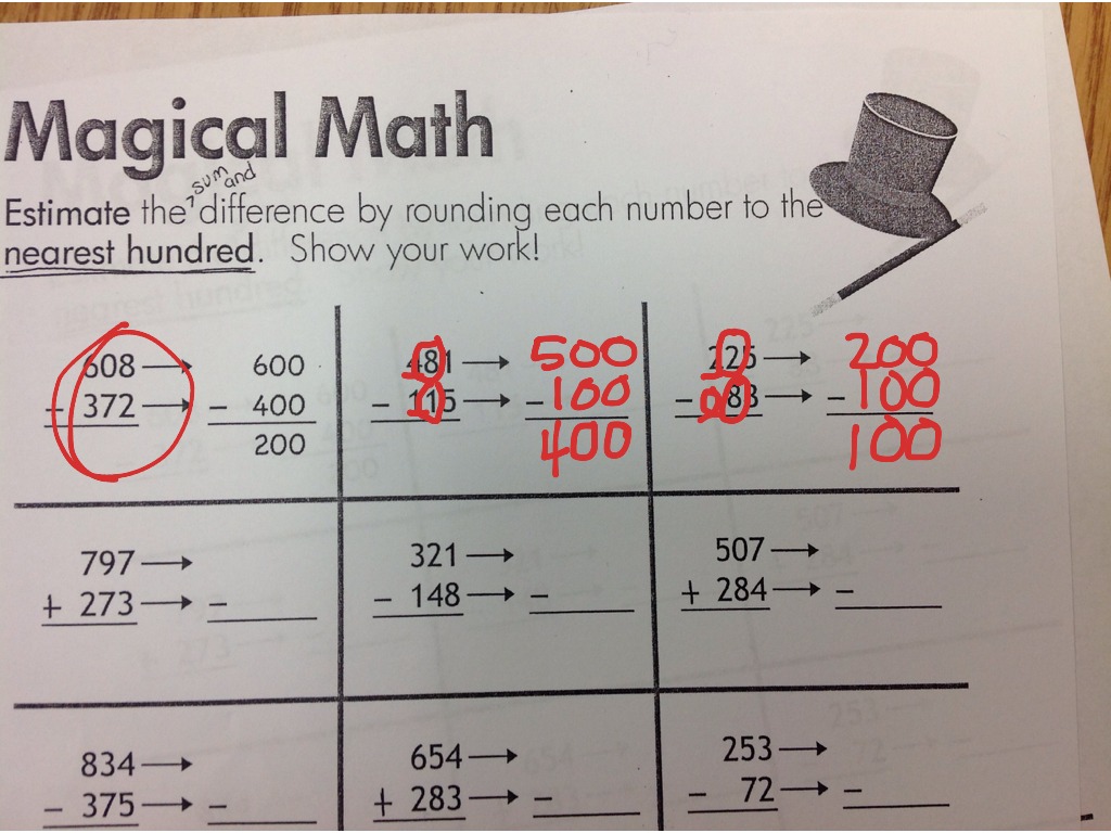 Hausdorff dimension.
Reminder of the last lecture
Hausdorff dimension
Dimension and measure of the Cantor set
Lecture 14. Lebesgue integral.
Hausdorff dimension of the Cantor set
Lebesgue integral
Properties of the Lebesgue integral
Chebyshev’s inequality
Lecture 15. Lebesgue’s theorem.
Reminder of the last lecture
Lebesgue’s theorem
Relationship between the Riemann integral and the Lebesgue integral
Variable substitution formula
Fubini’s theorem
Surface area formula
Lecture 16. Area formula.
Reminder of the last lecture
Area formula
Surface definition
Lecture 17. Application of the area formula.
Reminder of the last lecture
An example of applying the area formula
Definition of a piecewise smooth surface
Integration by parts formula
Lecture 18. Negligible sets.
Reminder of the last lecture
Properties of negligible sets
An example of negligible sets
Outer normal
Generalization of the Newton-Leibniz formula
Lecture 19. Sard’s theorem.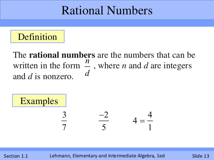
Unit splitting lemma
Sard’s theorem
Lecture 20. Coarea formula.
Reminder of the last lecture
Coarea formula
Rademacher’s theorem
Curvilinear integral of the second kind
Lecture 21. Differential 1 and 2-forms.
Reminder of the last lecture
Differential 1-form
Form transfer
Differential 2-form
Lecture 22. Transfer of the 2-form.
Poincaré’s lemma
Degree of circle-to-circle mapping
Statement 1
2-form transfer
Comment
Form Transfer Properties
Lecture 23.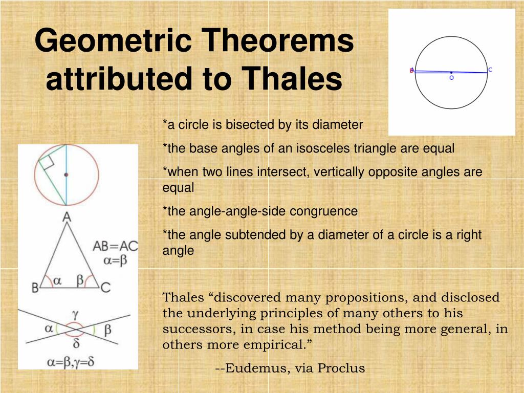 Surface integral of the second kind.
2-form integration
Surface integral of the second kind
Green’s formula in terms of differential forms
Stokes formula
Borsuk-Ulam theorem
Lecture 24. Geometric and physical interpretation of the external derivative.
Proof of the Borsuk-Ulam theorem
Geometric and physical interpretation of the external derivative
Gauss-Ostrogradsky formula
Stokes’ theorem
Lecture 25. Proof of the Gauss-Ostrogradsky formula.
Stokes formula
Proof of the Gauss-Ostrogradsky formula
Unit split
General proof case
KNOW INTUIT | Lecture | Logistics Decision Making Methodology
< Supplementary Material || Lecture 6 : 123
Keywords: structural analysis, morphological analysis, structural synthesis, parametric synthesis, model verification, adequacy assessment, isomorphic models, homomorphic models, pictorial model, functioning algorithm, optimality criterion, traveling salesman problem, demand flow, technological route, mathematical programming, maximum flow, linear programming problem
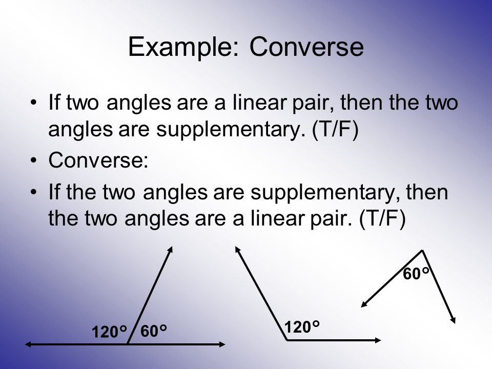 intuit.ru/2010/edi»> Methodology is the doctrine of the structure, logical organization, methods and means of activity. The modern theory of logistics is conceptually based on four methodologies: systems analysis (general systems theory), cybernetic approach (cybernetics), operations research , forecasting . Let us formulate a logical sequence of using the described scientific areas in the analysis, synthesis and optimization of drugs.
- LC with through flows moving along it objectively represents a complex or large LC, i.e. can be investigated by means of general systems theory .
- drugs are artificial, dynamic and targeted. For such systems, control problems, problems of analysis and synthesis of controlled and control systems are relevant, which can be studied, solved and modeled by methods of cybernetics .
- Any organizational and economic activity, and hence the management of logistics flow processes, is unthinkable without their long-term planning, without scientifically based forecasts of parameters and trends in the development of the external environment, indicators of logistics processes in drugs, etc. Such tasks are solved on the basis of methods and principles of forecasting .
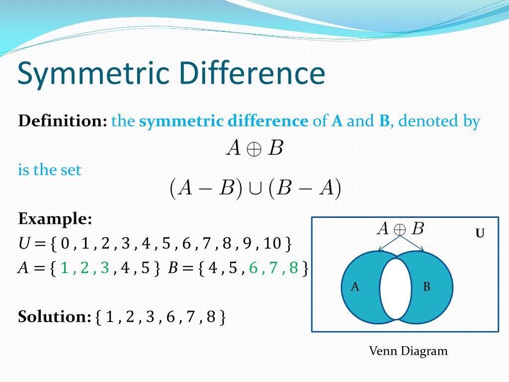 intuit.ru/2010/edi»> If we are talking about a control system, then there are problems of choosing the optimal solution and evaluating the effectiveness of control. The solution of these problems is provided by methods operations research .
5.1. Systems Analysis
General Systems Theory is a scientific discipline that develops methodological principles for the study of systems. The main feature of the general theory of systems in the approach to the objects of study as to systems .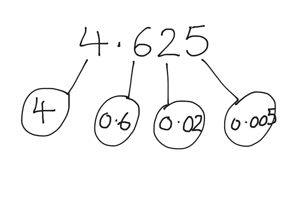
System analysis is a methodology of general systems theory, which consists in the study of any objects by representing them as systems, carrying out their structuring and subsequent analysis.
The main tasks of system analysis are:
- decomposition task means the representation of the system in the form of subsystems consisting of smaller elements;
- the task of analysis is to find various kinds of properties of the system, its elements and the environment in order to determine the patterns of system behavior;
-
the task of synthesis is to create a system model based on the knowledge about the system obtained in solving the first two problems, determine its structure, parameters that ensure the effective functioning of the system, solve problems and achieve goals.
The main functions of system analysis in the framework of the described three main tasks are presented in Table. 5.1.
| Structure of system analysis | ||
|---|---|---|
| Decomposition | Analysis | Synthesis |
| Definition and decomposition of the overall goal, the main function | Functional-structural analysis | Development of system model |
| Separating the system from the environment | Morphological analysis (component relationship analysis) | Structural synthesis |
| Description of influencing factors | Genetic analysis (history, trends, forecasting) | Parametric synthesis |
| Description of development trends, uncertainties | Analysis of analogues | System evaluation |
| Description as «black box» | Performance analysis | |
| Functional, component and structural decomposition | Formation of requirements for the system being created | |
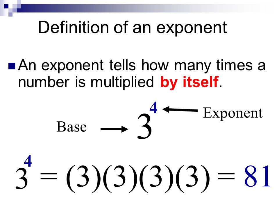 intuit.ru/2010/edi»> System analysis is based on a set of principles , i. provisions of a general nature, summarizing the experience of a person with complex systems. One of the main principles of system analysis is the principle of the ultimate goal , which consists in the absolute priority of the global goal and has the following rules:
- to conduct a system analysis, it is necessary first of all to formulate the main goal of the study;
- analysis should be carried out on the basis of understanding the main purpose of the system under study, which will determine its main properties, quality indicators and evaluation criteria;
- in the synthesis of systems, any attempt to change or improve the existing system must be evaluated in terms of whether it helps or hinders the achievement of the ultimate goal;
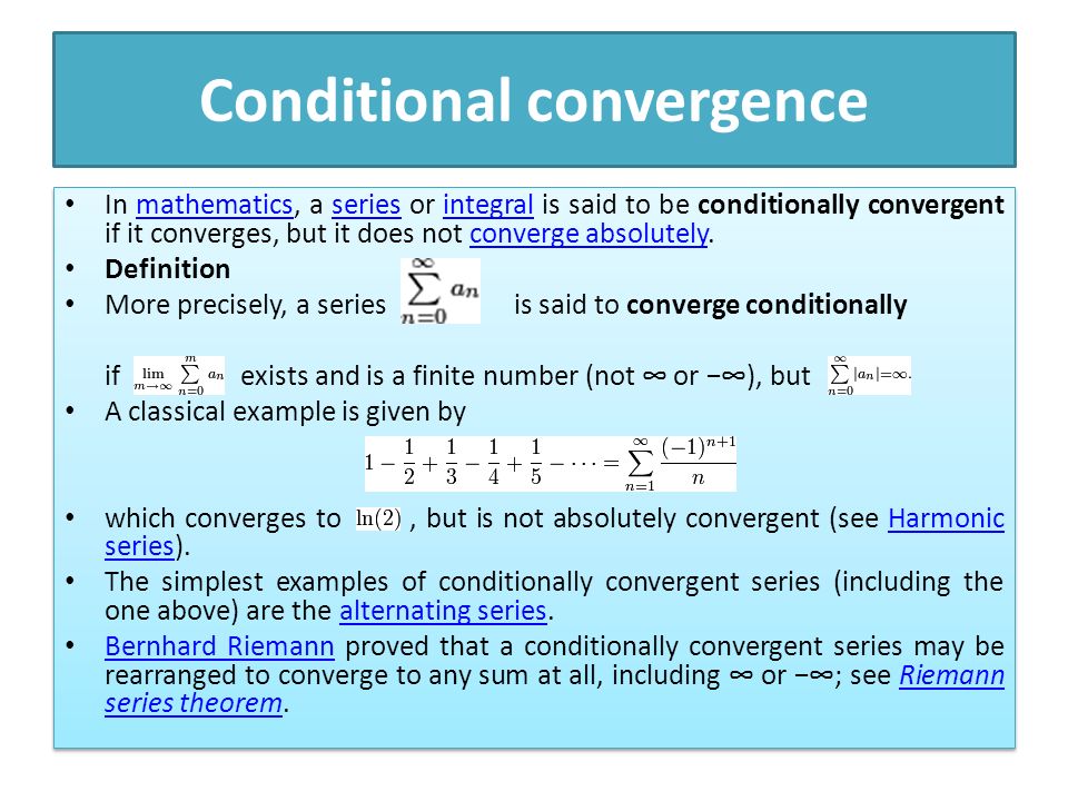 intuit.ru/2010/edi»> the purpose of the functioning of an artificial system is set, as a rule, by a system in which the system under study is an integral part.
The use of system analysis in logistics allows you to:
- determine and organize the elements, goals, parameters, tasks and resources of drugs, determine the structure of drugs;
- to identify the internal properties of drugs that determine its behavior;
- identify and classify relationships between elements of drugs;
- to identify unresolved problems, bottlenecks, uncertainties affecting the functioning, possible logistics activities;
- formalize semi-structured problems, reveal their content and possible consequences for entrepreneurs;
- to develop models that characterize the problem being solved from all the main sides and allow you to «lose» possible options for action, etc.
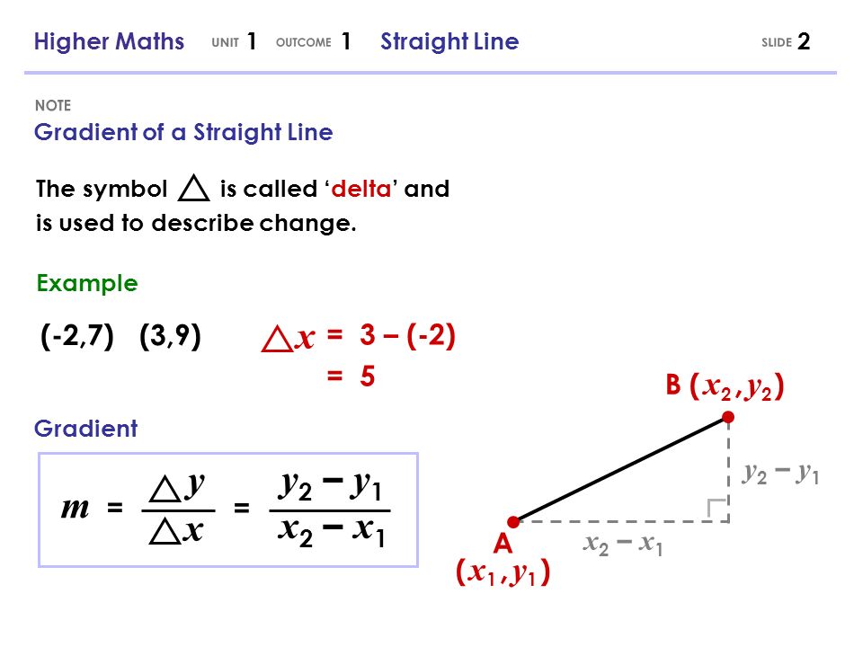 intuit.ru/2010/edi»> highlight the list and indicate the appropriate sequence for performing the tasks of the functioning of the drug and its individual elements;
5.2. Cybernetic approach
Cybernetics — the science of the general laws of control in nature, society, living organisms and machines, studying information processes associated with the control of dynamic systems. Cybernetic approach — study of a system based on the principles of cybernetics, in particular by identifying direct and feedback links, studying control processes, considering system elements as certain « black boxes «(systems in which only their input and output information is available to the researcher, and the internal structure may not be known).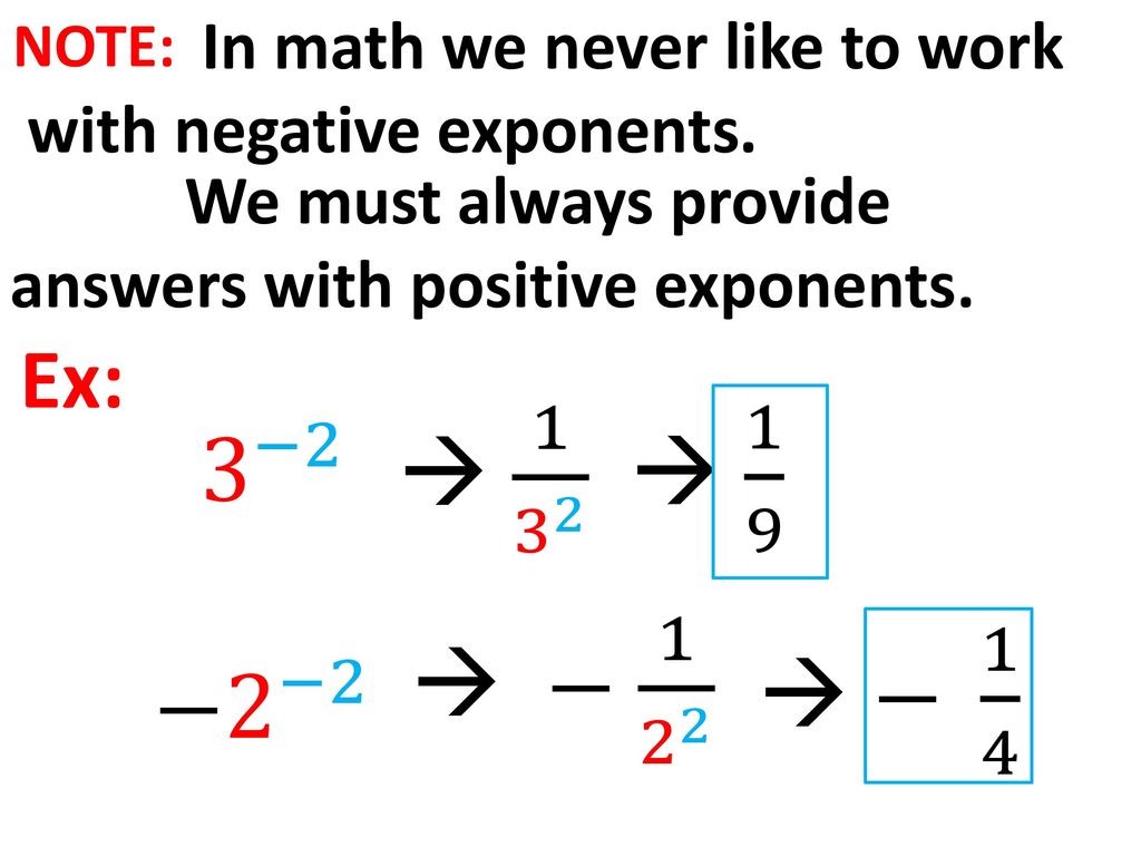
the structure and functions of systems, the study of control problems, etc. But unlike systems theory, cybernetics practices an informational approach to the study of control processes, which singles out and studies various types of information flows in the objects of study, ways of processing, analyzing, transforming, transmitting and etc. Management in its most general form is understood as the process of forming a purposeful behavior of the system through informational impact produced by a person or device.The following management tasks are distinguished:
- goal setting task — determination of the required state or behavior of the system;
- stabilization task — keeping the system in its current state under disturbing influences;
- the task of executing the program — transferring the system to the required state under conditions when the values of the controlled variables change according to known deterministic laws;
- optimization problem — keeping or transferring the system to a state with extreme values of characteristics under given conditions and restrictions.
 intuit.ru/2010/edi»>
tracking task — ensuring the required behavior of the system in conditions where the laws of change of controlled variables are unknown or change;
From the point of view of the cybernetic approach, the management of drugs is considered as a set of processes for the exchange, processing and transformation of information. The cybernetic approach represents the LAN as a system with control (Fig. 5.1), which includes three subsystems: the control system, the control object and the communication system.
enlarge image
Fig.
5.1.
Cybernetic approach to the description of LAN
 intuit.ru/2010/edi»> The control system together with the communication system forms a control system. The communication system includes a direct link channel through which input information {x} is transmitted and a feedback channel through which information about the state of the control object {y} is transmitted to the control system. Information about the controlled object and the environment is perceived by the control system, processed in accordance with a particular control goal, and transmitted to the control object in the form of control actions. The use of the concept of feedback is a distinctive feature of the cybernetic approach.
The main function groups of the control system are:
- decision-making functions or information content conversion functions are the main ones in the control system, expressed in the conversion of the content of information about the state of the control object and the environment into control information;
- information exchange functions are associated with bringing the developed solutions to the control object and the exchange of information between decision makers (collection, transmission of textual, graphic, tabular, electronic, etc. information by telephone, fax, local or global data networks, etc.). d.).
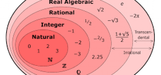 intuit.ru/2010/edi»>
routine information processing functions do not change the meaning of information, but cover only accounting, control, storage, search, display, replication, transformation of the form of information;
The application of the cybernetic approach to logistics requires the description of the basic properties of drugs using mathematical models. This makes it possible to develop and automate optimization algorithms for a cybernetic control system.
More >>
< Additional material || Lecture 6 : 123
Decision trees — CART mathematical apparatus.
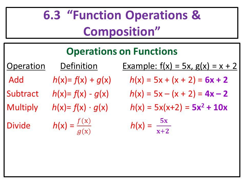 Part 1
The general principle of constructing decision trees was given in the article «Decision Trees — Basic Principles of Operation».
This article will focus on the CART algorithm. CART, short for Classification And Regression Tree, is a binary decision tree algorithm first published by Briman et al. at 1984 [1]. The algorithm is designed to solve classification and regression problems. There are also several modified versions — IndCART and DB-CART algorithms. The IndCART algorithm, which is part of the Ind package, differs from CART in using a different way of handling missing values, does not perform the regression part of the CART algorithm, and has different cutoff parameters. The DB-CART algorithm is based on the following idea: instead of using the training dataset to determine splits, use it to estimate the distribution of input and output values, and then use this estimate to determine splits. DB, respectively, means — «distribution based». This idea is claimed to result in a significant reduction in classification error compared to standard tree building methods.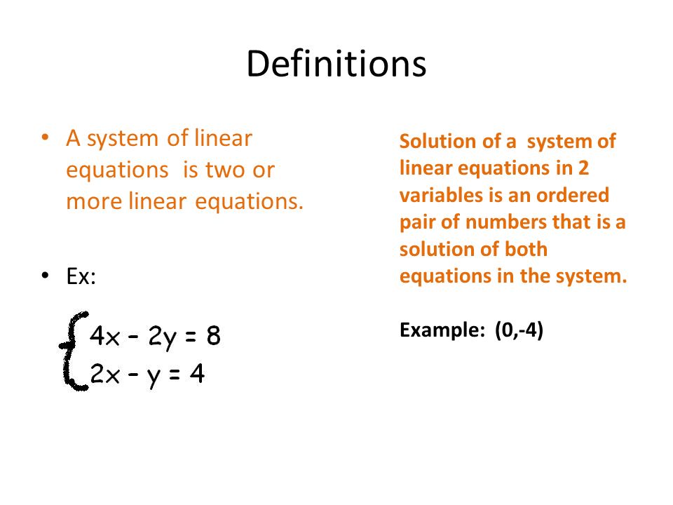
The main differences between the CART algorithm and the ID3 family algorithms are:
- binary representation of the decision tree;
- partition quality evaluation function;
- tree pruning mechanism;
- algorithm for handling missing values;
- building regression trees.
Binary representation of the decision tree
In the CART algorithm, each decision tree node has two children. At each step of building the tree, the rule formed in the node divides the given set of examples (training set) into two parts — the part in which the rule is true (child — right) and the part in which the rule is not true (child — left). To select the optimal rule, the function of estimating the quality of the partition is used.
Proposed algorithmic solution.
It is quite obvious. Each node (structure or class) must have references to two descendants Left and Right — similar structures. The node must also contain a rule identifier (for more details on the rules, see below), describe in some way the right side of the rule, contain information about the number or ratio of examples of each class of the training sample «passed» through the node, and have the sign of a terminal node — a leaf. These are the minimum requirements for the structure (class) of a tree node.
Partition quality evaluation function
Decision tree training refers to the supervised learning class, that is, training and test samples contain classified set of examples. The evaluation function used by the CART algorithm is based on the intuitive idea of reducing impurity (uncertainty) in a node. Consider a problem with two classes and a node that has 50 instances of one class each. The node has the maximum «impurity». If a partition is found that splits the data into two subgroups of 40:5 examples in one and 10:45 in the other, then intuitively the «impurity» will decrease. It will completely disappear when a split is found that will create subgroups 50:0 and 0:50. In the CART algorithm, the idea of »impurity» is formalized in index 92$ ,
where p i is the probability (relative frequency) of class i in T .
If the set T is divided into two parts T 1 and T 2 with the number of examples in each N 1 N 2 :
$$Gini_{split}\,(T) = \frac{N_1}{N}\,\cdot\,Gini\,(T_1)\,+\,\frac{N_2}{N}\, \cdot\,Gini\,(T_2)$$
The best split is the one for which Gini split (T) is minimal.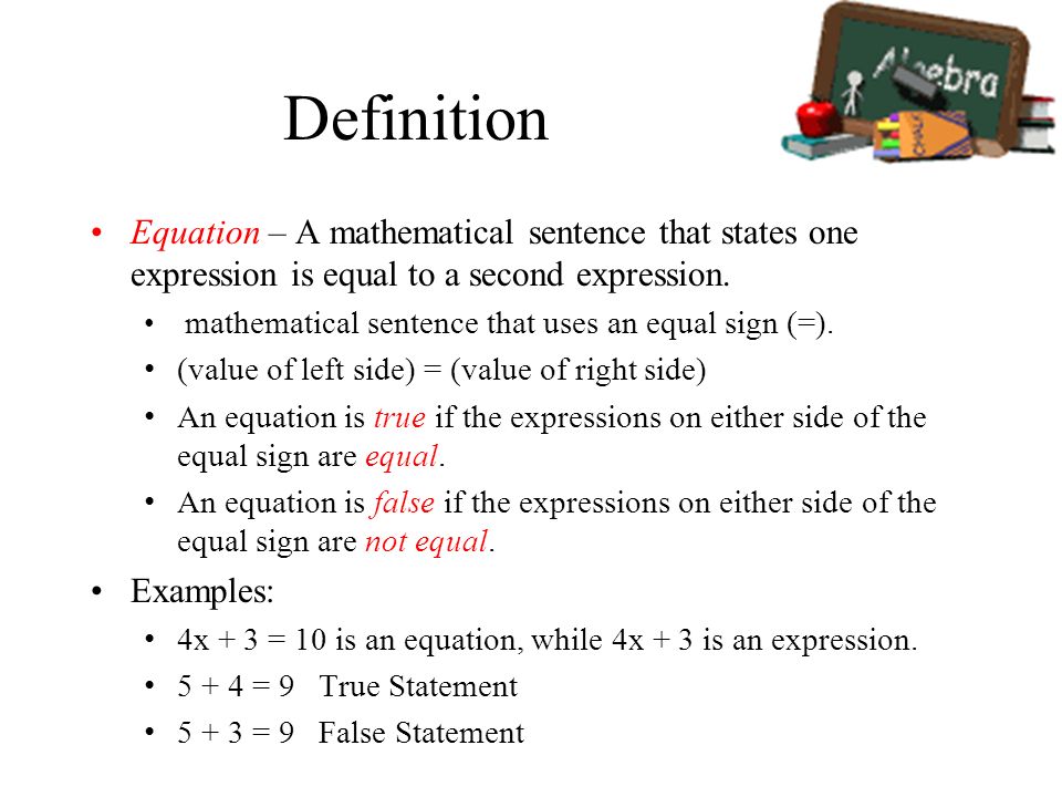 2\Biggr)\,\rightarrow\,\min$$ 92\rightarrow\max$$
As a result, the best partition is the one for which the value of is maximum . Less commonly, the CART algorithm uses other partitioning criteria Twoing, Symmetric Gini, etc., see [1] for more details.
Partitioning rules
The vector of predictor variables supplied to the input of the tree can contain both numeric (ordinal) and categorical variables. In any case, at each node, the partition goes only over one variable . If the variable is of a numeric type, then a rule of the form 9 is formed in the node0246 x i <= c . Where with is some threshold, which is most often chosen as the arithmetic mean of two adjacent ordered values of the variable x i of the training sample. If the variable is of categorical type, then the rule x i V(x i ) is formed in the node, where V(x i ) is some non-empty subset of the set of values of the variable x i in the training set.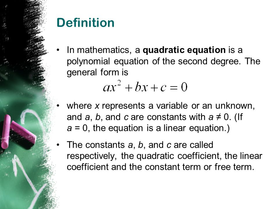 Therefore, for n values of a numeric attribute, the algorithm compares n-1 partitions, and for a categorical one (2 n-1 – 1). At each step of tree construction, the algorithm sequentially compares all possible partitions for all attributes and selects the best attribute and the best partition for it.
Proposed algorithmic solution.
Let’s agree that the source of the data necessary for the operation of the algorithm can be represented as a flat table. Each row of the table describes one example of a training/test set.
Each step of building a tree actually consists of a set of three laborious operations.
The first is sorting the data source by column. Required to calculate the threshold when the attribute currently being considered is of a numeric type. At each step of building a tree, the number of sorts will be at least equal to the number of attributes of a numeric type.
The second is the separation of the data source.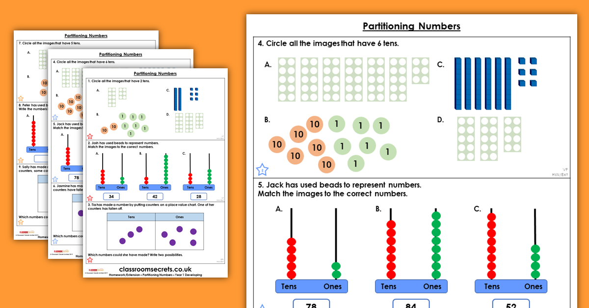 After the best partition is found, it is necessary to split the data source in accordance with the rule of the formed node and recursively call the construction procedure for the two halves of the data source.
Both of these operations are connected (if acted directly) with the movement of significant amounts of memory. Here, the data source is intentionally not called a table, since you can significantly reduce the time spent on building a tree if you use an indexed data source. Access to data in such a source occurs not directly, but through logical indexes of data rows. You can sort and split such a source with minimal performance loss.
The third operation, which takes 60–80% of the program execution time, is the calculation of indices for all possible partitions. If you have n — numeric attributes and m — examples in the sample, then you get a table of n * (m-1) — indexes, which takes up a large amount of memory. This can be avoided by using one column for the current attribute and one row for the best (maximum) indexes for all attributes.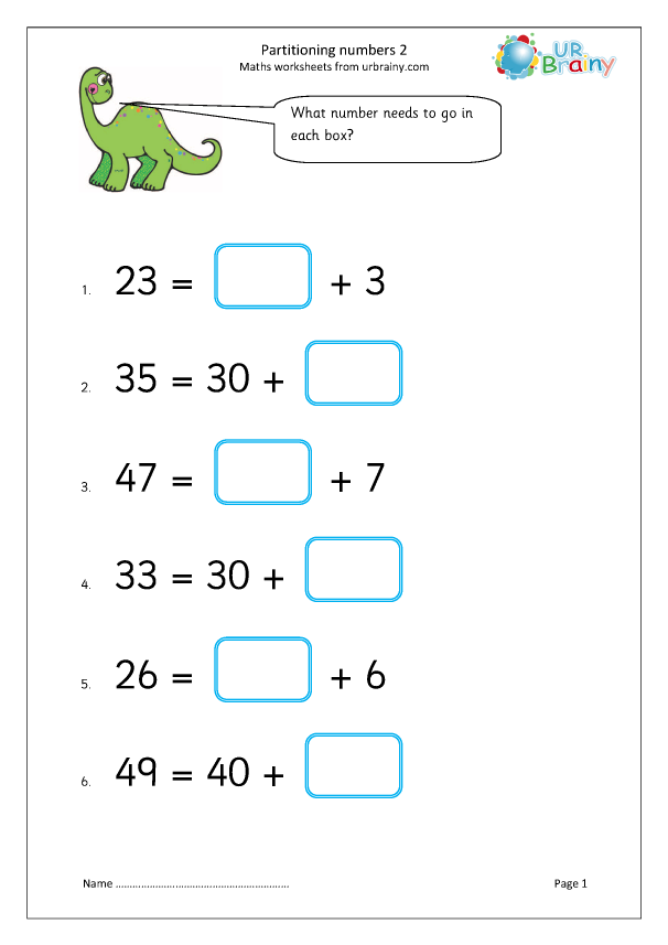 You can even use only a few numeric values, resulting in a fast, but poorly readable code. You can significantly increase productivity if you use that L \u003d N — R, l i = «n i » – r i , while l i and r i always change and only by one when moving to the next line for the current attribute. That is, counting the number of classes, and this is the main operation, will be performed quickly if you know the number of instances of each class in total in the table and, when moving to a new row in the table, change by one only the number of instances of one class — the class of the current example.
It is convenient to represent all possible partitions for categorical attributes by analogy with the binary representation of a number. If the attribute has n unique values. 2 n — partitions. The first (where all zeros) and the last (all ones) are of no interest to us, we get 2 n — 2. And since the order of the sets is also unimportant here, we get (2 n — 2) / 2 or (2 n- 1 — 1) the first (from one) binary representations. If {A, B, C, D, E} are all possible values of some attribute X, then for the current partition, which has a representation, say {0, 0, 1, 0, 1}, we obtain the rule X in {C, E} for the right branch and [ not {0, 0, 1, 0, 1} = {1, 1, 0, 1, 0} = X in {A, B, D} ] for the left branch.
Often, attribute values of a categorical type are represented in the database as string values. In this case, it is faster and more convenient to create a cache of all attribute values and work not with values, but with indexes in the cache.
Tree pruning
Tree pruning, originally called minimal cost-complexity tree pruning, is the most significant difference between the CART algorithm and other tree building algorithms. CART sees pruning as getting a compromise between two problems: getting an optimal tree size and getting an accurate estimate of the misclassification probability.
The main pruning problem is the large number of all possible pruned subtrees for a single tree.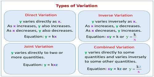 More precisely, if a binary tree has | T | – sheets, then there exists ~[1.5028369 |T| ] pruned subtrees. And if the tree has at least 1000 leaves, then the number of pruned subtrees becomes simply huge.
The basic idea of the method is not to consider all possible subtrees, limiting ourselves only to the «best representatives» according to the estimate below.
Denote | T | – number of tree leaves, R(T) – tree classification error equal to the ratio of the number of incorrectly classified examples to the number of examples in the training set. Let’s define $C_{\alpha}\,(T)$ – total cost (estimate/cost-complexity indicator) of the tree T as:
$C_{\alpha}\,(T) = R\,(T)\, +\,\alpha\,*\,|T|$, where | T | is the number of leaves (terminal nodes) of the tree, is some parameter that varies from 0 to + $\infty$. The total cost of a tree consists of two components — the tree classification error and the penalty for its complexity. If the classification error of a tree is constant, then as the value increases, the total cost of the tree will increase. Then, depending on , a less branched tree that gives a larger classification error may cost less than a tree that gives a smaller error, but more branched.
Define T max – the maximum size of the tree to be cut. If we fix the value of $\alpha$, then there is a smallest minimizable subtree $\alpha$ that satisfies the following conditions:
- $C_{\alpha}\Bigl(T\,(\alpha)\Bigr) = min_{\ ,\,T \leq T_{\max}}\,C_{\alpha}(T)$
- $if\,\,C_{\alpha}\,(T) = C_{\alpha}\Bigl(T\,(\alpha)\Bigr)\,then\,\,T\,(\alpha) \leq\,T$
The first condition says that there is no such subtree of the tree T max , which would have a lower cost than $T\,(\alpha)$ for this value of $\alpha$. The second condition says that if there is more than one subtree that has a given total cost, then we choose the smallest tree.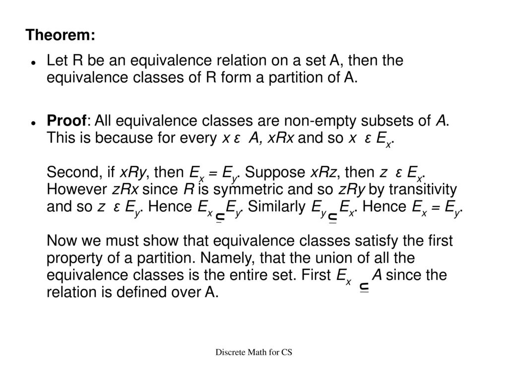
It can be shown that for any value there is such a smallest minimizable subtree. But this task is not trivial. What she is saying is that it cannot be that two trees reach a minimum total cost and they are incomparable, i.e. neither of them is a subtree of the other. We will not prove this result.
Although it has an infinite number of values, there are a finite number of subtrees of the tree Tmax. You can build a sequence of decreasing supports of the tree T Max :
T 1 > T 2 > T > …> {T 1 },
(where T 1 — tree root node) such that T k is the smallest minimizable subtree for $[\alpha_k,\,\alpha_{k+1})$. This is an important result, as it means that we can get the next tree in the sequence by applying pruning to the current tree. This allows us to develop an efficient algorithm for finding the smallest minimized subtree for various values of $\alpha$. The first tree in this sequence is the smallest subtree of the tree T max having the same classification error as T max , i. e. $T_1 = T(\alpha=0)$. Clarification: if the splitting goes on until only one class remains in each node, then T 1 = T max , but since prepruning methods are often used, then there may be a subtree of the tree T max having the same classification error.
Proposed algorithmic solution.
Calculation algorithm T 1 of T max simple Find any pair of leaves with a common ancestor that can be merged, i.e. truncated to the parent node without increasing the classification error. R(t) = R(l) + R(r) , where r and l are leaves of node t . Continue until there are no more pairs left. So we get a tree that has the same cost as T max at = 0, but less branching than T max .
How do we get the next tree in the sequence and the corresponding $\alpha$ value? Let T t be the branch of the tree T with the root node t .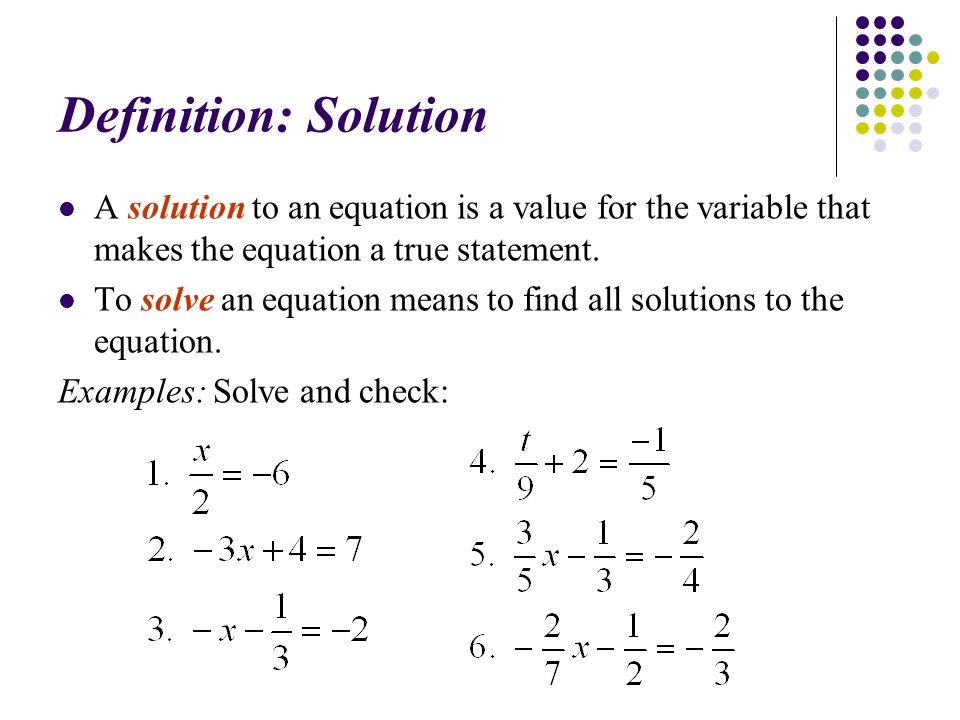 For what values will the tree T — T t be better than T ? If we cut at node t , then its contribution to the total cost of the tree T – T t becomes $C_{\alpha}(\{t\}) = R\,(t)\,+\, \alpha$, where R(t) = r(t)* p(t) , r(t) is the classification error of node t and p(t) is the proportion of cases that «passed» through node t . Alternative: R(t)= m/n , where m is the number of examples classified incorrectly, and n is the total number of classified examples for in a total of trees.
The contribution T t to the total cost of tree T is $C_{\alpha}(T_t) = R\,(T_t)\,+\,\alpha\,|T_t|$, where
$R\,(T_t) = \sum_{{t’}\in {T_t}}{R(t’)}$
Tree T – T t will be better than T when $C_{\alpha}\{(t\}) = C_{\alpha}\,(T_t)$, because with this they have the same value in magnitude, but T – T t is the smaller of the two.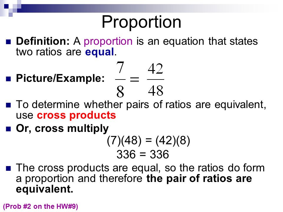 When $C_{\alpha}\{(t\}) = C_{\alpha}\,(T_t)$ we get:
$$R\,(T_t)\,+\,\alpha\,|T_t | = R\,(t)\,+\,\alpha$$
,(T_t)}{|T_t|\,-\,1}$$
So for any node t to T 1 if we increase $\alpha$ then when
$$\alpha = \frac{R\,(t)\,-\,R\ ,(T_{1,\,t})}{|T_{1,\,t}|\,-\,1}$$
the tree obtained by pruning at node t will be better than T 1 .
The main idea is the following: we calculate this value for each node in the tree T 1 , and then we select «weak ties» (there may be more than one), i.e. nodes for which the value is
$$g\,(t) = \frac{R\,(t)\,-\,R\,(T_{1,\,t})}{|T_{1,\,t} |\,-\,1}$$
is the smallest. We prune T 1 at these nodes to get T 2 , the next tree in the sequence. Then we continue this process for the resulting tree and so on until we get the root node (a tree with only one node).
Algorithm for computing a sequence of trees.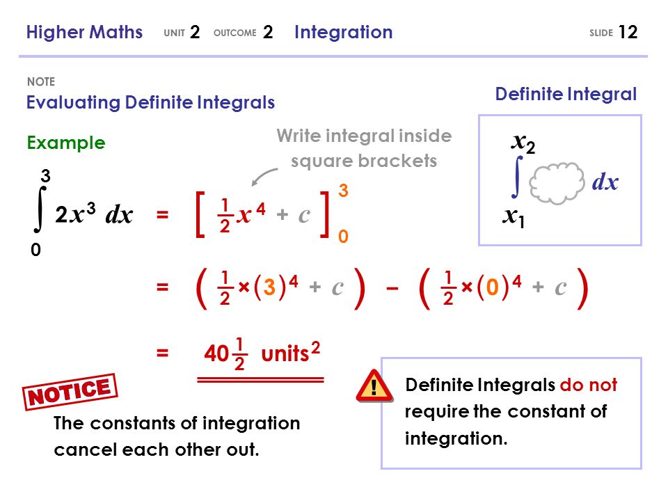
$T_1 = T\,(\alpha = 0)$
$\alpha_1 = 0$
k = 1
while T k > {root node} do begin
for all nonterminal nodes (!leaves) in t T k
$$g\,(t) = \frac {R\,(t)\,-\,R\,(T_{k,\,t})}{|T_{k,\,t}|\,-\,1}$$
$\alpha_{k+1} = min_{t}\,\,g_k(t)$
Traverse from top to bottom all nodes and truncate those where
$g_k(t) = \alpha_ {k+1}$
k = k + 1
end
Nodes must be traversed from top to bottom in order not to cut off nodes that are cut off by themselves, as a result of cutting off the n-th ancestor.
Consider the method in more detail using an example.
As an example, let’s calculate the sequence of subtrees and corresponding values for the tree shown in fig. 1.
Obviously, T 1 = T max , since all sheets contain examples of the same class and cutting off any node ( t 3 or t 5 9250 leads to an increase in the error) 5 925 classification.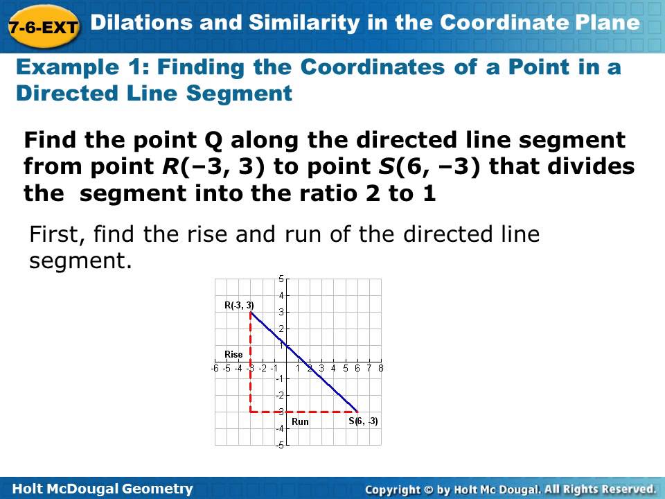
Then we calculate g 1 (t) for all units t to t 1 .
$$g\,(t_1) = \frac{R\,(t_1)\,-\,R\,(T_{1,\,t_1})}{|T_{1,\,t_1}| \,-\,1}$$
R(t 1 ) – classification error. If we turn t 1 into a leaf, then some class should be associated with it; since the number of examples of both classes is the same (equal to 100), then the class is chosen at random, in any case it incorrectly classifies 100 examples. In total, the tree was trained on 200 examples (100+100=200 for the root node). R(t 1 ) = m/n. m=100, n=200. R(t 1 ) = 1/2.
$R\,(T_1,\,t_1)$ is the sum of errors of all leaves of subtree . It is counted as the sum over all sheets of the ratio of the number of misclassified examples in sheet to the total number of examples for in tree . In the example, we divide everything by 200. Since for the subtree rooted at t 1 , it is the same tree T 1 , all leaves do not have misclassified examples, so 95\frac{0}{200} = 0$$
$|T_1,\,t_1|$ number of leaves of subtree rooted at node t 1 .![]() There are 5 in total.
There are 5 in total.
We get:
g 1 (t 1 ) = (1/2 — 0)/(5 — 1) = 1/8.
g 1 (t 2 ) = 3/20.
g 1 (t 3 ) = 1/20.
g 1 (t 5 ) = 1/20.
Nodes t 3 and t 5 both store the minimum value g 1 , we get a new tree T 2 by cutting T 1 at both these nodes. We got the tree shown in Figure 2.
Next, we continue to calculate g -value for T 2 .
g 2 (t 1 ) = (100/200 — (0/200 + 10/200 + 10/200)) / (3 — 1) = 2/10.
g 2 (t 2 ) = (60/200 — (0/200 + 10/200)) / (2 — 1) = 1/4.
The minimum is stored at node t 1 , so we truncate at t 1 and get the root of the tree (T 3 = {t 1 0 } This completes the cutting process.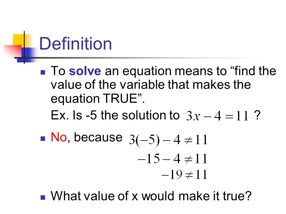
The sequence of values is: $\alpha$ 1 = 0, $\alpha$ 2 = 1/20, $\alpha$ 3 = 2/10 . So T 1 is the best tree for [0, 1/20) , T 2 — for [1/20, 2/10) and
Selection of the final tree
So, we have a sequence of trees, we need to choose the best tree from it. The one we will use in the future. The most obvious is the choice of the final tree through testing on a test set. The tree with the lowest classification error is the best tree. However, this is not the only possible way.
For a continuation of the description, see the article «Description of the CART algorithm. Part 2».
Literature
- L. Breiman, J.H. Friedman, R.A. Olshen, and C.T. Stone. Classification and Regression Trees. Wadsworth, Belmont, California, 1984.
- J.R. Quinlan. C4.5 Programs for Machine Learning. Morgan Kaufmann, San Mateo, California, 1993.
- Machine Learning, Neural and Statistical Classification.